
"Liberation Day" tariffs: market response to the announcement and court ruling
This study examines factor rankings and portfolio outcomes around two tariff events: the April 2, 2025 announcement of the tariff schedule and the February 20, 2026 Supreme Court ruling that removed its legal basis. It follows the response across sectors, assets, and probability-weighted portfolios.
Companies' import dependence, pricing power, supply chains, and balance sheets create different exposures to a tariff change. Evaluating factor scores and subsequent returns around both events helps assess whether those differences provided useful evidence for portfolio construction.
The April announcement established a 10% additional duty on most imports and higher country-specific rates. Over the following week, retaliation between the United States and China intensified before the administration suspended the higher country-specific rates for most trading partners on April 9. The 10% rate remained in place, while the additional rate on Chinese imports rose to 125%, bringing the effective rate on many Chinese goods to 145%. The S&P 500 rose 9.5% on the day of the pause. That gain left the index below its April 2 close.
Ten months later, the Supreme Court ruled 6-3 in Learning Resources, Inc. v. Trump that the International Emergency Economic Powers Act grants the president no authority to impose tariffs. The administration signed a replacement 10% surcharge under Section 122 of the Trade Act of 1974 that day, with effect from February 24. The S&P 500 gained 0.7% on the day of the ruling.
Each window contains several policy actions as well as concurrent market news. The reported factor scores and returns combine all of those events. A tariff-only causal estimate would require a different research design.
Event windows and data
The April window runs from the April 2 close, when the tariff schedule was announced, through the April 9 close. It therefore includes the initial selloff, China's retaliation, the escalation in US tariffs on Chinese goods, and the relief rally after the 90-day pause. The February window runs from the February 19 close through February 26, covering the ruling and the first two trading days after the replacement surcharge took effect.
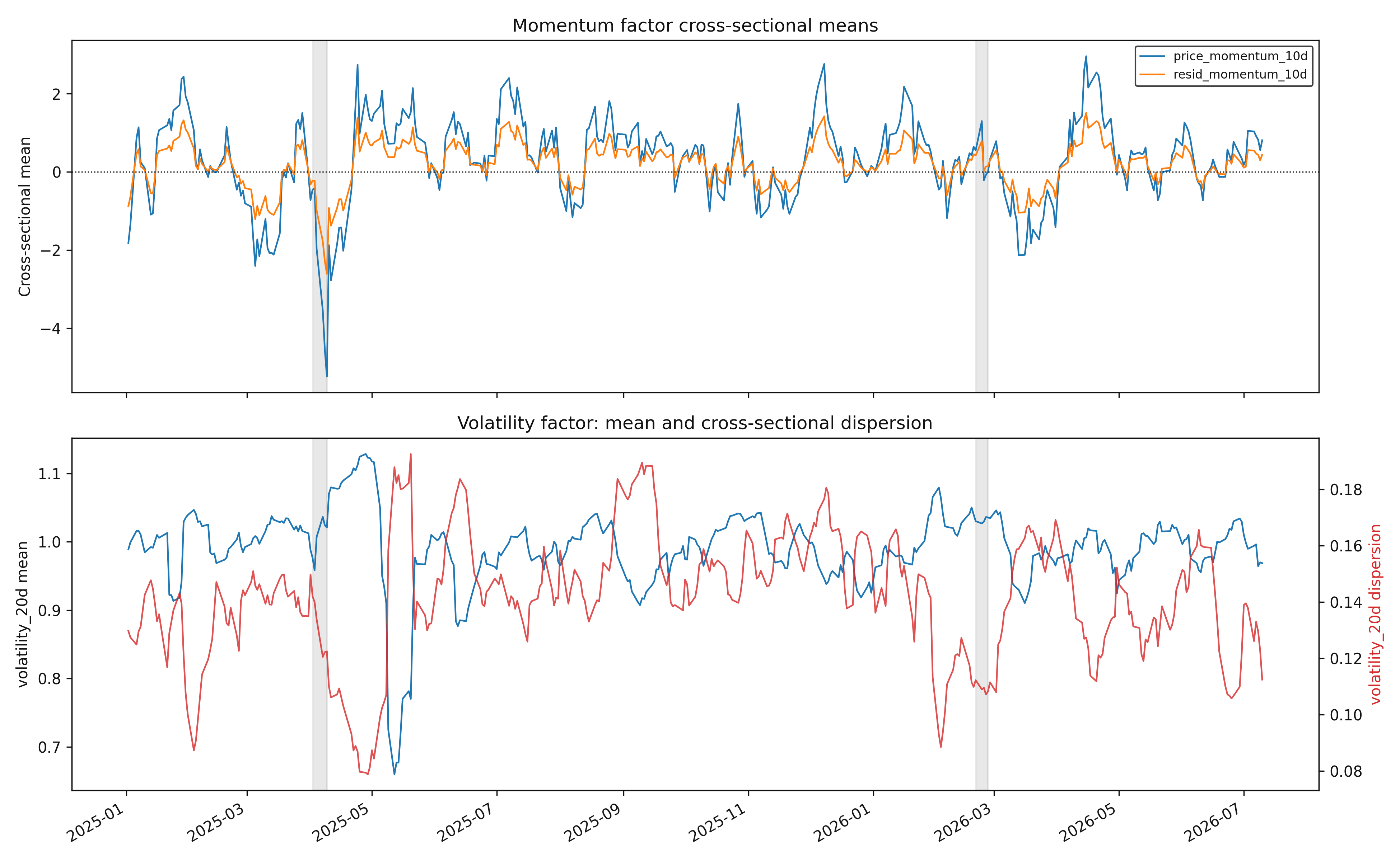
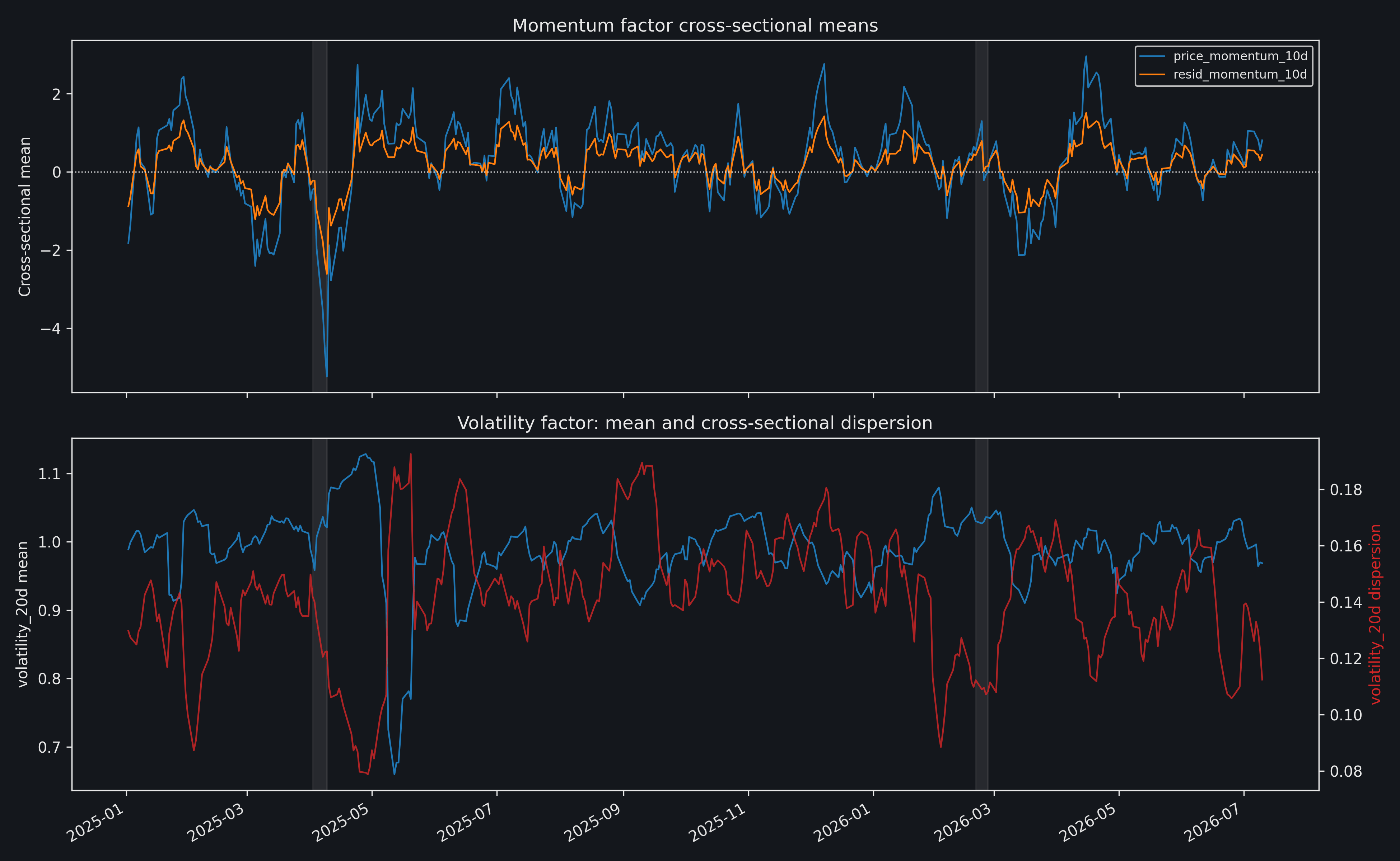
The factor series are daily cross-sectional aggregates of production scores for US equities from January 2, 2025 through July 10, 2026. Figure 1 reports the mean scores for 10-day price momentum and residual momentum, together with the mean and cross-sectional standard deviation of the 20-day volatility score. ETF returns in Figures 2 and 3 are split-adjusted, close-to-close returns over each event window. The available factor universe grows from roughly 1,750-1,850 securities during the April window to about 2,050 during the February window, changing the composition of the cross-sectional statistics across dates.
Factor response
Both momentum means fell sharply in April. From April 3 through April 9, the 10-day price-momentum mean fell from -0.42 to -5.24 and residual momentum from -0.22 to -2.61. Those April 9 values were the sample lows. Each score uses trailing 10-day returns, so the April 9 reading includes the preceding selloff and that day's rally.
The same measures changed much less in February. From February 20 to February 26, the price-momentum mean moved from 0.55 to approximately zero, while the residual-momentum mean moved from 0.42 to 0.15. Both changes fall within the range of other fluctuations in the series.
From April 3 to April 9, the mean volatility score rose modestly from 0.96 to 1.02, while its cross-sectional standard deviation narrowed from 0.140 to 0.123. That combination indicates more uniform volatility scores across the equity universe. Dispersion reached its sample minimum later, at 0.079 on April 29. The February window produced little change in either measure.
Sector returns
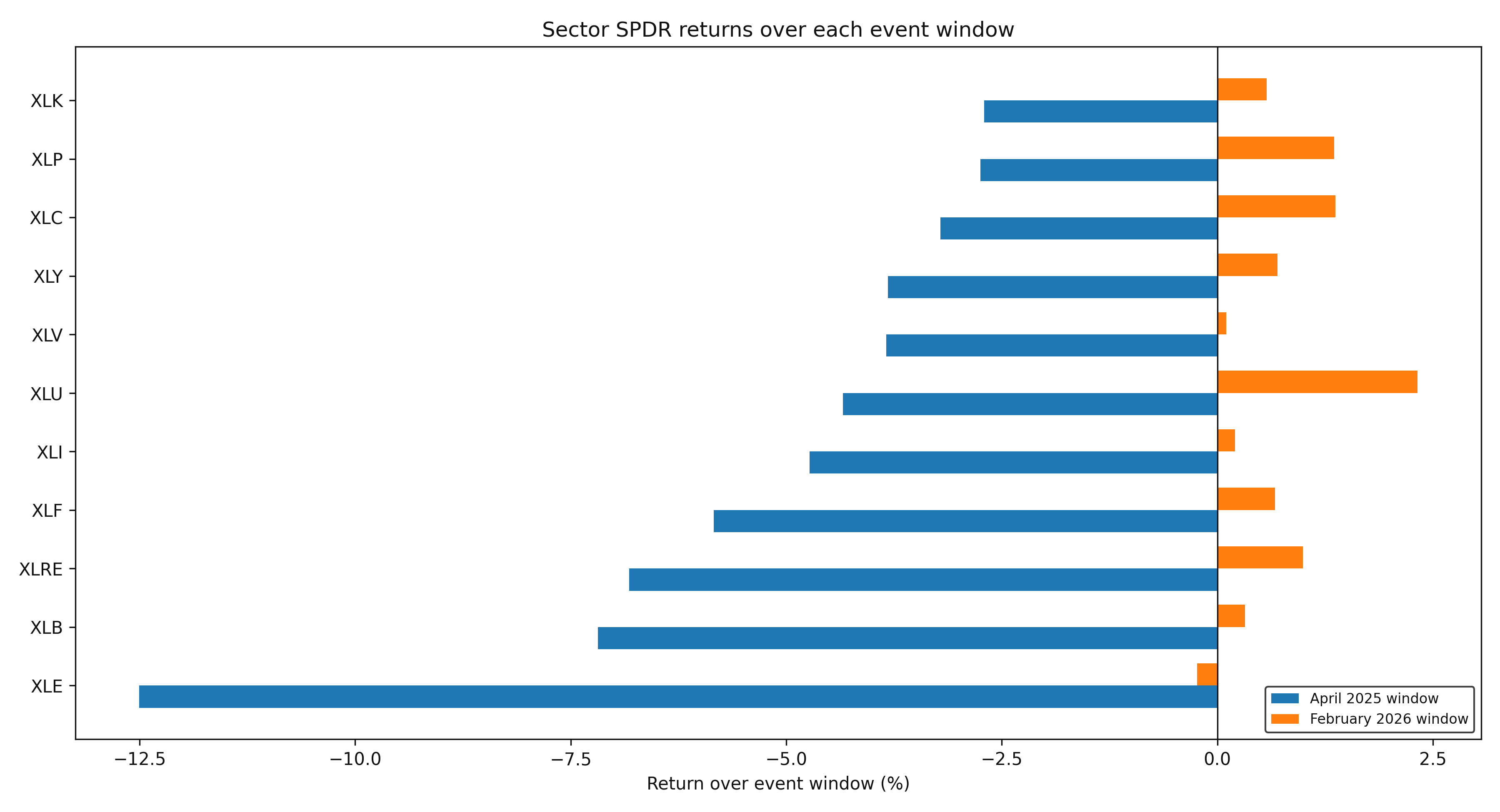
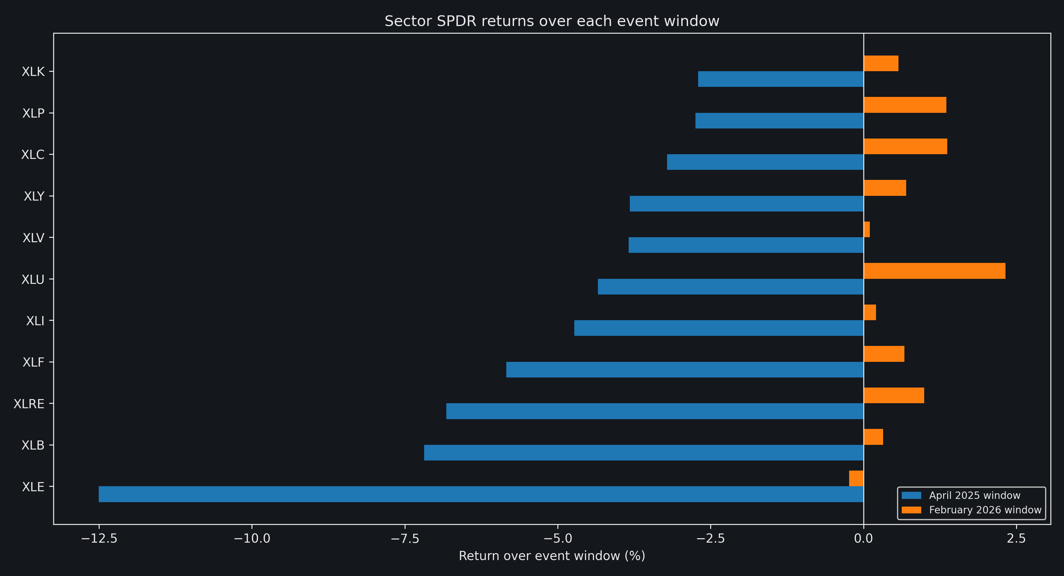
All eleven sector SPDRs had negative returns over the April window, even after the April 9 rally. Energy (XLE) was the weakest at -12.5%. Materials (XLB) lost 7.2% and real estate (XLRE) lost 6.8%, while technology (XLK) had the smallest decline at 2.7%. The declines covered sectors with both high and low direct exposure to imported goods.
In February, ten sector ETFs gained. Utilities (XLU) led at 2.3%, while energy (XLE) was the sole decline at 0.2%.
Cross-asset returns
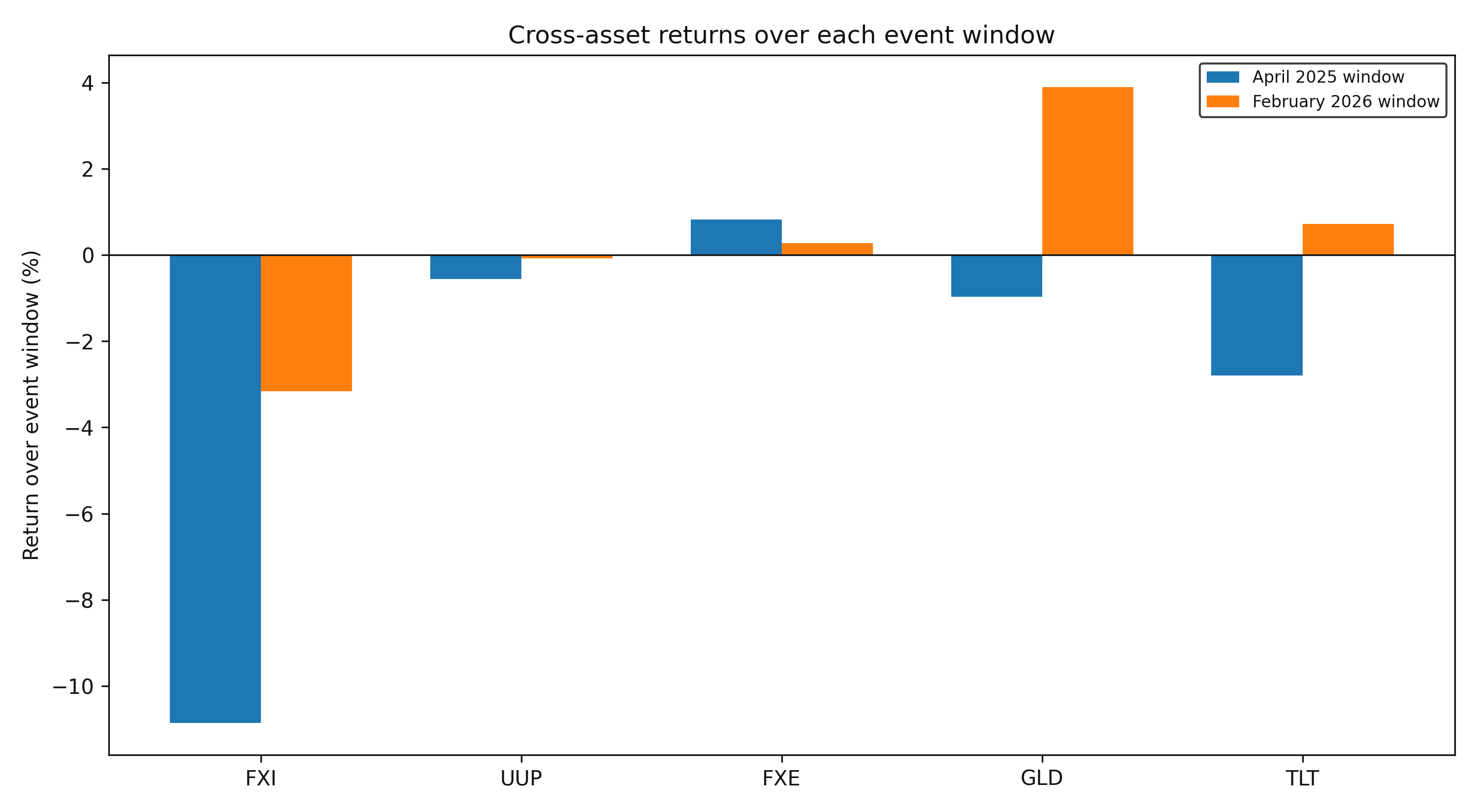
FXI fell 10.9% in April and 3.2% in February, the largest decline in each window. Treasuries and gold reversed direction: TLT fell 2.8% in April and rose 0.7% in February; GLD fell 1.0% and rose 3.9%. UUP declined 0.6% and 0.1%, while FXE gained 0.8% and 0.3%. The February window contained other macro developments, so attributing the gold move would require a separate analysis.
Probability-weighted tariff portfolios
The historical April comparison begins at the April 2 close, when the tariff schedule was released. The trading exercise begins one session earlier, at the April 1 close. Its five-session horizon ends on April 8, before the April 9 pause changed the policy path.
The conditional view assumes a broad tariff announcement with a large China component and weaker growth expectations. The five-session payoff inputs are
Conditional five-session excess returns used in the tariff view
| Asset | Conditional excess return |
|---|---|
| FXI | -8.0% |
| XLE | -5.0% |
| XLB | -4.0% |
| SPY | -5.0% |
| XLP | -2.0% |
| XLU | -2.0% |
| GLD | +2.0% |
| TLT | +1.0% |
The assumed returns are specified before evaluation. Prices through April 1 supply the covariance estimate; later prices are used only to evaluate the allocations.
Two mandates express the same view. The long-only mandate chooses among SPY, a defensive portfolio (50% XLP and 50% XLU), a haven portfolio (50% GLD and 50% TLT), and cash. The overlay mandate chooses among three fully collateralized, unit-gross positions:
china_short: short FXI;cyclical_short: 50% short XLE and 50% short XLB; andhaven_vs_spy: 25% long GLD, 25% long TLT, and 50% short SPY.
Residual overlay weight remains as cash collateral. Each active position has unit gross exposure; because active position weights sum to at most one, look-through gross exposure is capped at 100%.
Let \(v\) denote the conditional excess-return vector and \(p\) the probability assigned to the tariff view. The baseline state assigns every risky position the cash return, so \(v\) is its excess return in the tariff state. Each run uses
\[\mu(p) = r_f\mathbf{1} + p v,\]
\[\Sigma(p) = \Sigma_{\mathrm{pre}} + p(1-p)vv^\top.\]
The covariance estimate uses 60 daily observations from January 2 through April 1 and is scaled to five sessions. Cash uses the 4.32% three-month Treasury yield on April 1. The mean-variance solver uses a risk-aversion coefficient of 30. Realized overlay returns include the collateral return. Borrow costs, trading costs, collateral haircuts, taxes, and distributions are set to zero.
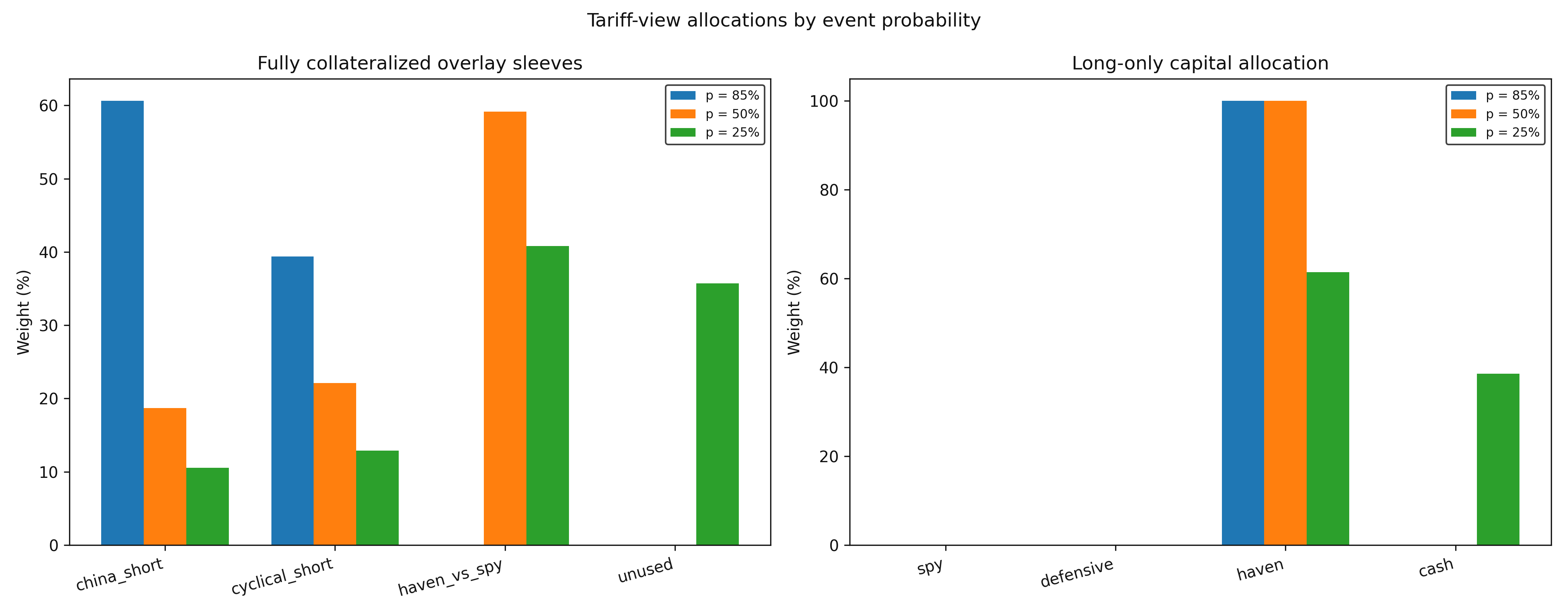
At 85%, the overlay holds 60.6% in the China short and 39.4% in the cyclical short. At 50%, it holds 18.7% in the China short, 22.1% in the cyclical short, and 59.1% in the haven-versus-SPY position. At 25%, unused overlay capacity rises to 35.7%.
The long-only mandate allocates fully to the haven portfolio at 85% and 50%. At 25%, it holds 61.5% in the haven portfolio and 38.5% in cash. The negative conditional returns on SPY and the defensive portfolio lead the solver to assign zero weight to both.
Forecast statistics and subsequent portfolio returns
| Mandate | View probability | Expected 5d return | Expected 5d vol | April 8 | April 9 |
|---|---|---|---|---|---|
| Overlay | 85% | 5.7% | 3.6% | +17.0% | +10.7% |
| Overlay | 50% | 2.3% | 2.7% | +9.2% | +4.4% |
| Overlay | 25% | 0.8% | 1.5% | +5.6% | +2.6% |
| Long only | 85% | 1.4% | 1.4% | -3.9% | -1.8% |
| Long only | 50% | 0.8% | 1.5% | -3.9% | -1.8% |
| Long only | 25% | 0.3% | 0.9% | -2.3% | -1.1% |
Equities sold off through April 8: FXI lost 17.3%, while XLE and XLB lost 18.7% and 13.9%. GLD and TLT also lost 4.3% and 3.4%. The long-only haven portfolio therefore declined, while the short and relative overlays earned positive returns.
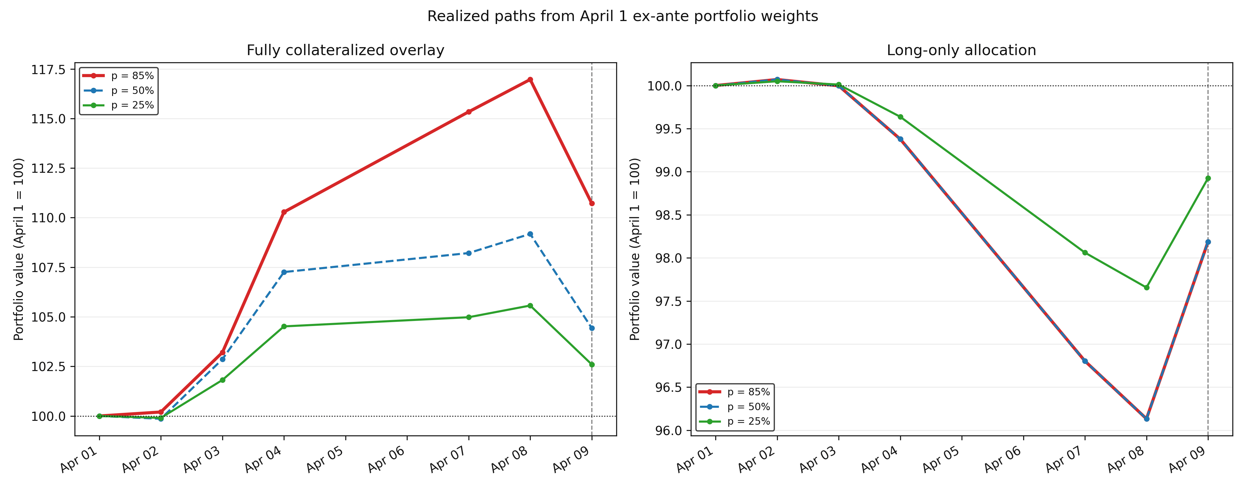
The weights remain fixed throughout Figure 5. After the April 9 rally, overlay gains fell and the long-only loss narrowed. A dynamic allocation would set a new event probability and payoff vector after each policy update, then trade at the next executable price.
Event-window comparison and portfolio outcomes
April produced larger changes in the factor statistics and ETF returns reported here. Both momentum means reached their sample lows, all eleven sector ETFs declined, and four of the five cross-asset proxies moved by more than they did in February. The court-ruling window brought smaller factor changes and modest sector returns.
By February 2026, lower courts had already rejected the use of IEEPA for the tariffs, giving investors months to assess the prospect of an adverse Supreme Court decision. The replacement surcharge preserved a broad import tax under a different statute. The April 2025 announcement, meanwhile, supplied the first country-level schedule and was followed by several revisions in one week.
Higher event probabilities increased exposure and changed the mix of positions. The long-only mandate moved toward havens and lost money because both haven proxies fell. Under the overlay mandate, the China and cyclical shorts produced positive P&L from the same tariff assumptions.
This walkthrough is for research and educational purposes. It illustrates how strategynet.ai organizes signal evidence into factors and scenarios. It provides no recommendation, investment advice, or instruction to trade any security.
Back to Insights