
What mean-variance optimization misses about joint losses
Portfolio losses can concentrate when several investments share an economic exposure. Mean-variance optimization represents their joint behavior through covariance; maximum-loss and historical CVaR penalties give explicit weight to adverse joint-return scenarios. This study examines how those penalties change the allocation among related factor-mimicking portfolios.
The study compares five allocation rules, then evaluates the nominal and CVaR objectives over the same finite set of portfolios. That comparison isolates the effect of the joint-loss penalty from the numerical method used to select weights, helping researchers assess how the risk objective affects holdings.
Allocation inputs
The allocator estimates an expected-return score and covariance matrix from rolling samples. The ICIR score uses the mean and dispersion of each FMP's recent information coefficients. The covariance matrix uses a separate rolling return window. Historical scenario rows retain the joint return of every FMP on each date.
Related FMPs can hold many of the same securities, producing high correlations and simultaneous losses. Covariance and joint-loss scenarios describe that dependence across the candidate portfolios.
Problem formulation
For \(n\) candidate FMPs, let
- \(w \in \mathbb{R}^{n}\) be the vector of FMP allocation weights;
- \(\alpha \in \mathbb{R}^{n}\) be their allocation scores;
- \(\Sigma \in \mathbb{R}^{n \times n}\) be their annualized covariance matrix; and
- \(R \in \mathbb{R}^{S \times n}\) contain \(S\) historical return scenarios.
The feasible set is
\[\mathcal{W} = \left\{ w \in \mathbb{R}^{n} : \mathbf{1}^{\mathsf T}w=1,\; \ell_i \leq w_i \leq u_i \right\}.\]
The budget applies to the candidate columns supplied to the allocator. Cash or a market allocation requires its own candidate column. The empirical run below contains six FMPs and allocates the full budget among them. Each FMP can contain long and short constituent positions even though its allocation weight is non-negative.
ICIR allocation score
The service uses the FMP construction-weight IC when that series is available. For construction \(i\) on date \(t\), let \(x_{i,t}\) denote its vector of constituent weights and let \(r_{t+1}\) denote the corresponding next-period returns. The cross-sectional statistic is
\[\operatorname{IC}_{i,t} = \operatorname{corr}_{\mathrm{rank}} \left(x_{i,t},r_{t+1}\right).\]
This measures the rank association between the positions produced by the FMP construction and the subsequent constituent returns. Over a trailing window of \(T\) observations, the annualized ICIR is
\[\operatorname{ICIR}_{i} = \sqrt{A}\, \frac{\overline{\operatorname{IC}}_{i}} {s\left(\operatorname{IC}_{i}\right)},\]
where \(A=252\) and \(s(\cdot)\) is the sample standard deviation. The mean-variance allocator uses
\[\alpha_i = c\,\operatorname{ICIR}_i,\]
with \(c=0.01\) in the current service. This scaling produces an allocation score. A separate calibration is required to interpret it as an expected FMP return. Window length and the value of \(c\) therefore enter the economic interpretation of \(\lambda\) in the optimization.
Covariance estimate
Let \(r_t\) be the vector of FMP returns at observation \(t\). Over a window of \(T\) observations, the service estimates
\[\widehat{\Sigma} = \frac{A}{T-1} \sum_{t=1}^{T} \left(r_t-\bar r\right) \left(r_t-\bar r\right)^{\mathsf T}.\]
Portfolio variance, \(w^{\mathsf T}\widehat{\Sigma}w\), reflects the variance of each FMP, its covariance with the other FMPs, and its weight. A lower-scoring FMP can reduce total variance when its covariance with the existing allocation is sufficiently low.
Short histories and closely related FMPs can produce a poorly conditioned matrix. Shrinkage, factor covariance models, and longer windows are possible extensions; the run below uses the sample covariance directly.
Nominal mean-variance allocation
The nominal allocator solves
\[\underset{w \in \mathcal{W}}{\operatorname{maximize}} \quad \alpha^{\mathsf T}w - \frac{\lambda}{2} w^{\mathsf T}\widehat{\Sigma}w.\]
The parameter \(\lambda>0\) scales estimated variance relative to the ICIR score. Smaller values permit greater concentration in high-scoring FMPs. Larger values favor lower estimated variance. The weight bounds cap the allocation to any one FMP.
With the budget and box constraints removed, the first-order solution is
\[w^{*} = \frac{1}{\lambda} \widehat{\Sigma}^{-1}\alpha.\]
If \(\widehat{\Sigma}=QDQ^{\mathsf T}\), then
\[w^{*} = \frac{1}{\lambda} \sum_{j=1}^{n} \frac{q_j q_j^{\mathsf T}\alpha}{d_j}.\]
Directions with small eigenvalues \(d_j\) receive large multipliers. Estimation errors in \(\alpha\) and \(\widehat{\Sigma}\) can therefore move the solution most along low-eigenvalue directions. Box constraints limit position size.
Historical joint-loss scenarios
For historical scenario \(s\), let \(r_s\) denote the simultaneous return of every FMP. The portfolio loss is
\[L_s(w)=-r_s^{\mathsf T}w.\]
Each scenario row comes from the trailing covariance window available at the rebalance date. Simultaneous FMP losses enter \(L_s(w)\) together.
Maximum-loss penalty
The maximum observed portfolio loss is
\[L_{\max}(w) = \max\left(0,\max_{1\leq s\leq S}L_s(w)\right).\]
The service adds its squared, annualized value to the variance term:
\[\underset{w \in \mathcal{W}}{\operatorname{maximize}} \quad \alpha^{\mathsf T}w - \frac{\lambda}{2} \left[ w^{\mathsf T}\widehat{\Sigma}w + \eta A L_{\max}(w)^2 \right].\]
Here \(\eta \in [0,1]\) controls the historical loss contribution. The date with the largest portfolio loss determines the penalty.
CVaR penalty
The CVaR mode averages the largest losses in the selected tail. Sort the scenario losses from largest to smallest,
\[L_{(1)}(w) \geq L_{(2)}(w) \geq \cdots \geq L_{(S)}(w),\]
and for confidence level \(q\) define
\[m=\left\lceil(1-q)S\right\rceil, \qquad \widehat{\operatorname{CVaR}}_{q}(w) = \frac{1}{m} \sum_{j=1}^{m}L_{(j)}(w).\]
The service sets
\[T_q(w) = \max\left( 0, \widehat{\operatorname{CVaR}}_{q}(w) \right)\]
and solves
\[\underset{w \in \mathcal{W}}{\operatorname{maximize}} \quad \alpha^{\mathsf T}w - \frac{\lambda}{2} \left[ w^{\mathsf T}\widehat{\Sigma}w + \eta A T_q(w)^2 \right].\]
At \(q=0.95\), a full 126-observation scenario window produces a seven-observation tail. The first three allocations in this run used expanding scenario windows of 63, 84, and 105 observations, producing tail counts of four, five, and six. Every allocation in the reporting interval used 126 scenarios.
Finite-grid solution
The maximum-loss and CVaR modes enumerate feasible simplex points and select the highest objective value. In the reported configuration, a 10 percentage-point step, six FMPs, and a 50% per-FMP cap produce 2,247 feasible portfolios. A smaller step increases the number of candidates. The service stops after 250,000 evaluations and returns the best point in that enumerated prefix. The current 2,247-point grid is evaluated in full. A larger step reduces the available weight choices.
Setting robust.weight to zero sends the service to the continuous nominal
solver. The research script constructs the grid-matched nominal benchmark from
the archived FMP histories and the service's grid enumeration order.
Run configuration
Configuration used for the allocator comparison
| Setting | Value |
|---|---|
| Candidate FMPs | Six constructions of alpha_cs_model_v1 |
| ICIR window | 63 aligned observations |
| Covariance and scenario window | Up to 126 aligned observations |
| Rebalance cadence | Every 21 aligned observations |
| Risk aversion | lambda = 2.0 |
| HRP and mean-variance bounds | 0% to 50% per FMP |
| CVaR settings | q = 0.95; eta = 0.5 |
| Robust grid | 10 percentage points; 2,247 feasible portfolios |
| Allocation cost | 5 bp per unit of L1 allocation-weight change |
The trailing-ICIR benchmark clips negative ICIR values to zero and normalizes the remaining scores. This permits weights above the 50% cap applied to HRP and mean-variance. Its largest FMP allocation reached 52.65% before the reporting interval. Equal weight remains fixed at one-sixth per FMP.
Allocation methods
Inputs used by each allocation method
| Method | Allocation score | Covariance | Historical tail |
|---|---|---|---|
| Equal weight | None | None | None |
| Trailing ICIR | Positive rolling ICIR | None | None |
| Hierarchical risk parity | None | Sample covariance | None |
| Nominal mean-variance | Rolling ICIR | Sample covariance | None |
| CVaR-robust mean-variance | Rolling ICIR | Sample covariance | Empirical CVaR |
Walk-forward comparison
The candidate set contains full-universe equal and z-score weighting, equal-weight 10%, 20%, and 33% tails, and z-score-weighted 10% tails. Every candidate uses the same cross-sectional signal. Each allocator received the same dated FMP return and construction-weight IC histories.
The data request covers 9 July 2024 through 9 July 2026. The aligned candidate matrix contains 476 observations beginning 10 July 2024. The dynamic methods begin on 8 October 2024 after the 63-observation ICIR warm-up and produce 413 return observations. The aligned history jumps from 2 January to 13 February 2025, a 42-calendar-day gap retained in the history. The reporting interval lies after the gap.
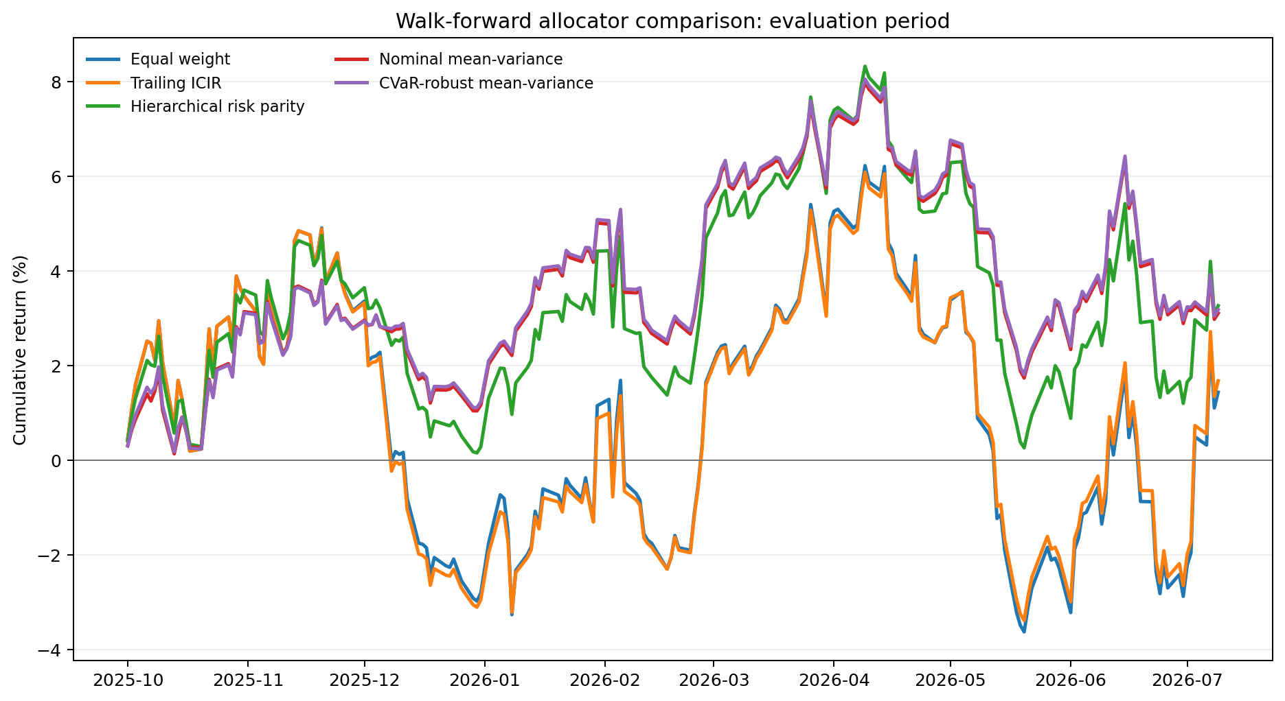
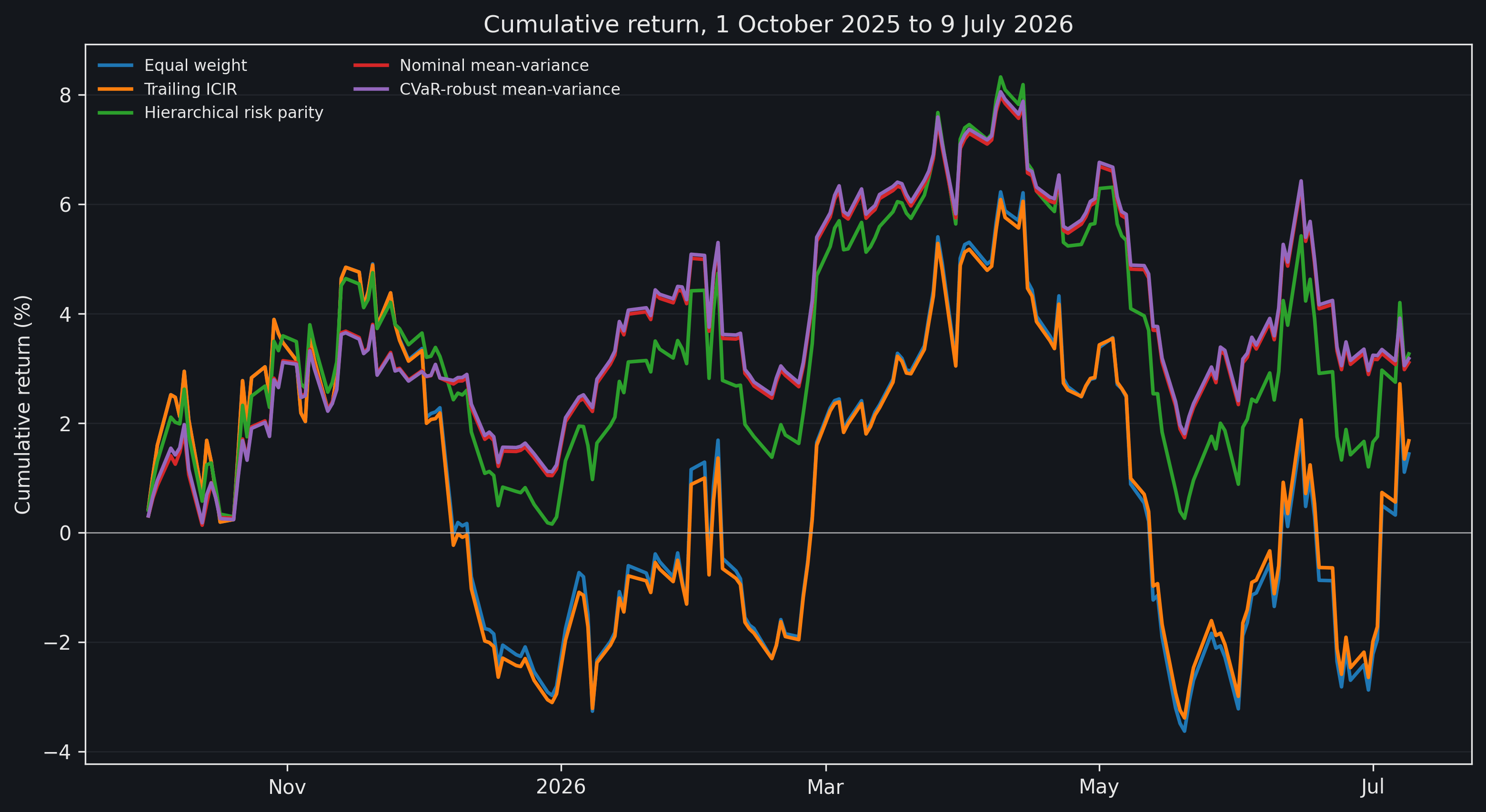
The reporting interval runs from 1 October 2025 through 9 July 2026 and contains 195 observations. The interval label was added on 10 July 2026, after the period ended. The split is retrospective and the results are descriptive.
Weights use information available before each rebalance observation and remain in force until the next rebalance. Rebalancing occurs every 21 aligned observations. The first three covariance estimates use 63, 84, and 105 observations; all later estimates use the full 126-observation window.
Reporting-interval performance, 1 October 2025 to 9 July 2026
| Method | Annualized return | Sharpe (0% cash rate) | Max drawdown |
|---|---|---|---|
| Equal weight | 1.86% | 0.21 | 9.28% |
| Trailing ICIR | 2.17% | 0.24 | 8.93% |
| Hierarchical risk parity | 4.24% | 0.48 | 7.45% |
| Nominal mean-variance | 4.04% | 0.56 | 5.78% |
| CVaR-robust mean-variance | 4.13% | 0.58 | 5.78% |
Nominal and CVaR-robust mean-variance followed similar paths. Their charted difference contains the continuous-versus-grid solver choice; the matched-grid calculation below attributes the CVaR term.
Matched-grid attribution
At each CVaR rebalance, the research script evaluates the nominal objective over the same 2,247 portfolios used by the CVaR method. It also reconstructs the service's selected CVaR weights. The reconstruction matches all 20 archived allocation snapshots to machine precision.
Nominal and CVaR selections on the same 10% grid
| Period | Rebalances | Same selection | Different selection |
|---|---|---|---|
| Before 1 October 2025 | 11 | 6 | 5 |
| Reporting interval | 9 | 9 | 0 |
The tail penalty changed the grid selection on 19 September 2025, the allocation carried into the reporting interval. The nominal grid selected 50% full-universe equal weight and 50% 33% tails. CVaR selected 50% full-universe equal weight, 10% full-universe z-score weight, and 40% 33% tails. Both objectives selected the same 50/50 grid portfolio on 20 October and at the remaining eight rebalances.
The inherited September allocation affected returns through 19 October. The 20 October rebalance moved 10% of capital, recorded 20% L1 turnover, and incurred a 1 bp charge. Figure 1 also includes the finer weights from the continuous nominal solver.
Reporting-interval allocation diagnostics
| Method | Annualized L1 turnover | Average HHI | Mean capital reallocated |
|---|---|---|---|
| Equal weight | 0.00 | 0.167 | 0.0000 |
| Trailing ICIR | 1.64 | 0.172 | 0.0704 |
| Hierarchical risk parity | 0.42 | 0.250 | 0.0182 |
| Nominal mean-variance | 0.06 | 0.499 | 0.0025 |
| CVaR-robust mean-variance | 0.26 | 0.495 | 0.0111 |
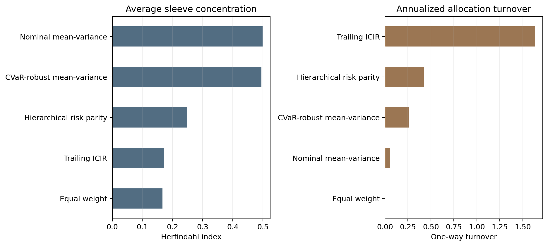
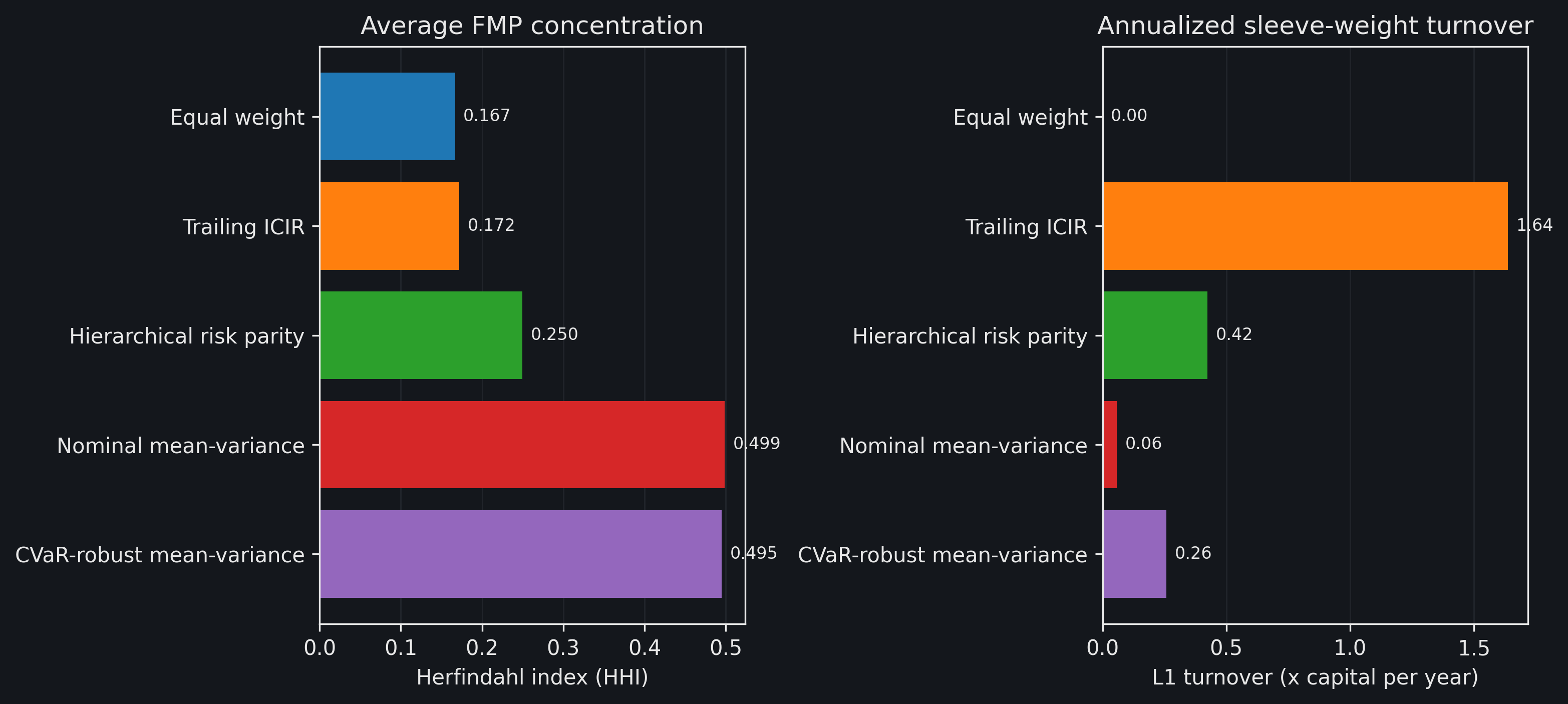
Average HHI near 0.5 for both mean-variance methods reflects sustained concentration in roughly two FMPs at the 50% cap. The CVaR-robust method's September-to-October change also accounts for part of its higher turnover.
Event-view application
An event thesis can enter the allocation through state-dependent FMP return estimates and probabilities set at the decision date. All estimates must use a common horizon and return units. Let \(\mu_k\) and \(\Sigma_k\) be the conditional FMP mean vector and covariance matrix in state \(k\), and let \(p_k\) be its probability. The mixture mean is
\[\bar\mu(p) = \sum_k p_k \mu_k,\]
and the law of total covariance gives
\[\Sigma(p) = \sum_k p_k \left[ \Sigma_k + \left(\mu_k-\bar\mu(p)\right) \left(\mu_k-\bar\mu(p)\right)^{\mathsf T} \right].\]
The view-adjusted portfolio solves, for example,
\[\underset{w \in \mathcal{W}}{\operatorname{maximize}} \quad \bar\mu(p)^{\mathsf T}w - \frac{\lambda}{2}w^{\mathsf T}\Sigma(p)w - \kappa C(w,w_0),\]
where \(C(w,w_0)\) represents the cost of moving from the pre-event portfolio. Using the rolling-ICIR score in this objective requires a calibration from \(\alpha\) into the same return units as \(\mu_k\).
Running the optimizer over a probability grid produces \(w(p)\), the ex-ante portfolio path as confidence in the thesis changes. A discrete set of state-contingent return scenarios and probabilities defines the loss distribution for CVaR. For a binary event, a probability set \(\mathcal{P}=\{p:p_L\leq p\leq p_U\}\), with \(0\leq p_L\leq p_U\leq1\), defines a max-min allocation over the plausible values of \(p\). For each probability, report the FMP weights, changes from the pre-event portfolio, expected return, volatility, turnover, and binding constraints. Time-stamped inputs establish which assumptions were available at the decision date.
Limitations
This comparison covers one signal, six related constructions, one reporting interval, and one parameter set. Constituent-level costs and cross-FMP trade netting are outside its scope. The results should therefore be tested across different ICIR and covariance windows, objective parameters, tail thresholds, and grid resolutions before they are generalized.
Further reading
- What Is Alpha Uncertainty?. How forecast-error covariance changes the robust value assigned to an expected-return estimate.
- How Do Multiple Risk Models Enter Portfolio Construction?. How covariance blends and separate risk limits treat disagreement between competing estimates.
- From Information Coefficient to Portfolio Weights. The complete mapping from signal calibration through covariance-aware, cost-aware portfolio construction.
- Harry Markowitz, "Portfolio Selection",
The Journal of Finance, 1952. - R. Tyrrell Rockafellar and Stanislav Uryasev,
"Optimization of Conditional Value-at-Risk",
The Journal of Risk, 2000. - Victor DeMiguel, Lorenzo Garlappi, and Raman Uppal,
"Optimal Versus Naive Diversification: How Inefficient Is the 1/N Portfolio Strategy?",
The Review of Financial Studies, 2009. - Marcos Lopez de Prado,
"Building Diversified Portfolios that Outperform Out of Sample",
The Journal of Portfolio Management, 2016.
This walkthrough is for research and educational purposes. It illustrates how strategynet.ai organizes signal evidence into factors and scenarios. It provides no recommendation, investment advice, or instruction to trade any security.
Back to Insights