
US-Israel/Iran conflict (Feb 28 – Mar 9, 2026): from factor shock to a risk-adjusted portfolio
This study examines factor scores, sector prices, energy markets, and prediction-market probabilities around the 2026 US–Iran conflict. It uses StrategyNet's production data and factor panel, together with Polymarket's public price history, to assess how a stated energy-market view and its uncertainty translate into portfolio holdings and realized outcomes.
The analysis connects the market response to the sizing decision. It traces which exposures the factor evidence identified and how portfolio construction affected the return earned during the event window.
Joint US-Israeli strikes on Iranian leadership and military infrastructure began Saturday, February 28, 2026, with the first trading-day reaction on Monday, March 2. Iran retaliated against US bases in Jordan, UAE, and Qatar. Oil broke $100/bbl for the first time since 2022 on March 9, on roughly 7 million barrels/day of projected regional shut-in risk. Tensions continued well past the initial event window, into July 2026.
Background: refining capacity was already tight
U.S. refining capacity remains large by global standards, but it is below its recent peak: operable crude-distillation capacity is roughly 18.1–18.2 million barrels per day, down about 700,000– 800,000 b/d from the 2020 high following several permanent refinery closures. The system has less structural spare capacity than it did before the pandemic, even though the refineries that remain have generally become more efficient and capable of running at high rates.
Refinery utilization rose sharply as the market moved into the summer driving season. Rates that were near 89–91% before and shortly after the conflict increased into the mid-90s by June, with some weekly readings around 96–97%, near the practical upper limit for the national system. Although a 96% utilization rate appears to leave 4% unused, much of that residual reflects maintenance, outages, and units that are technically operable but not immediately available. As a result, the throughput that could realistically be brought online is considerably smaller than the headline spare-capacity figure suggests.
Domestic gasoline demand followed its normal seasonal pattern, rising from winter levels as spring and summer travel increased. Product supplied moved from roughly 8.5 million barrels per day before the conflict to approximately 8.9 million barrels per day afterward. Refiners initially increased gasoline production enough to meet much of this increase, but the rise in output was smaller than the normal seasonal production ramp by early summer. Inventories consequently declined faster than usual, moving from above their five-year seasonal average before the conflict to materially below average by July.
Exports remain an important part of the balance. The U.S. continued to export roughly 0.9–1.0 million barrels per day of gasoline, primarily from the Gulf Coast, even while importing gasoline and blending components into the East Coast. This reflects regional infrastructure and shipping economics rather than a national shortage: the Gulf Coast is structurally long refining capacity, while the East Coast is relatively short and often relies on imports from Europe and Canada. The system overall remained capable of meeting domestic demand, but was doing so with high utilization, reduced inventory cover, and limited room to absorb a major refinery outage or a further increase in demand.
Data
The factor panel contains daily cross-sectional aggregates for four production signals: 10-day price momentum, 10-day residual momentum, 20-day volatility, and a 10-day return z-score. Changes in equity coverage over the sample affect the daily means and standard deviations.
Prices are split-adjusted closes from September 2, 2025 through July 10, 2026. They measure price return and exclude distributions. The historical event return begins at the February 27 close, the final session before the Saturday strikes, and ends at the March 9 close. That interval contains six trading sessions. The intraday series uses regular-session prices in Eastern time. A matched September-to-July period from the prior year provides one seasonal reference.
Factor evolution
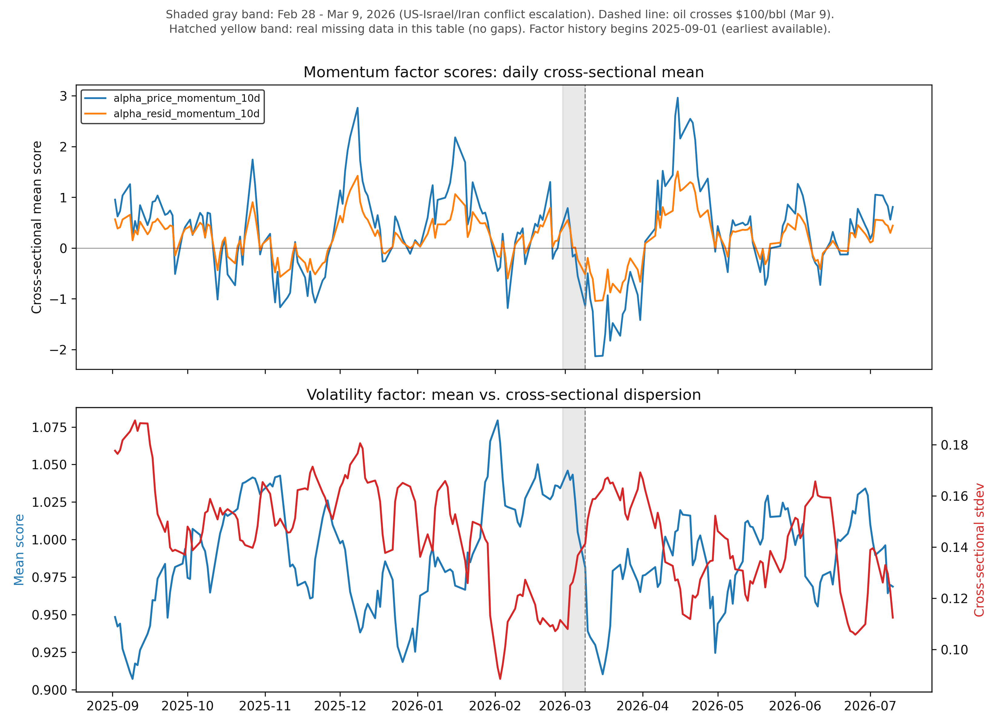
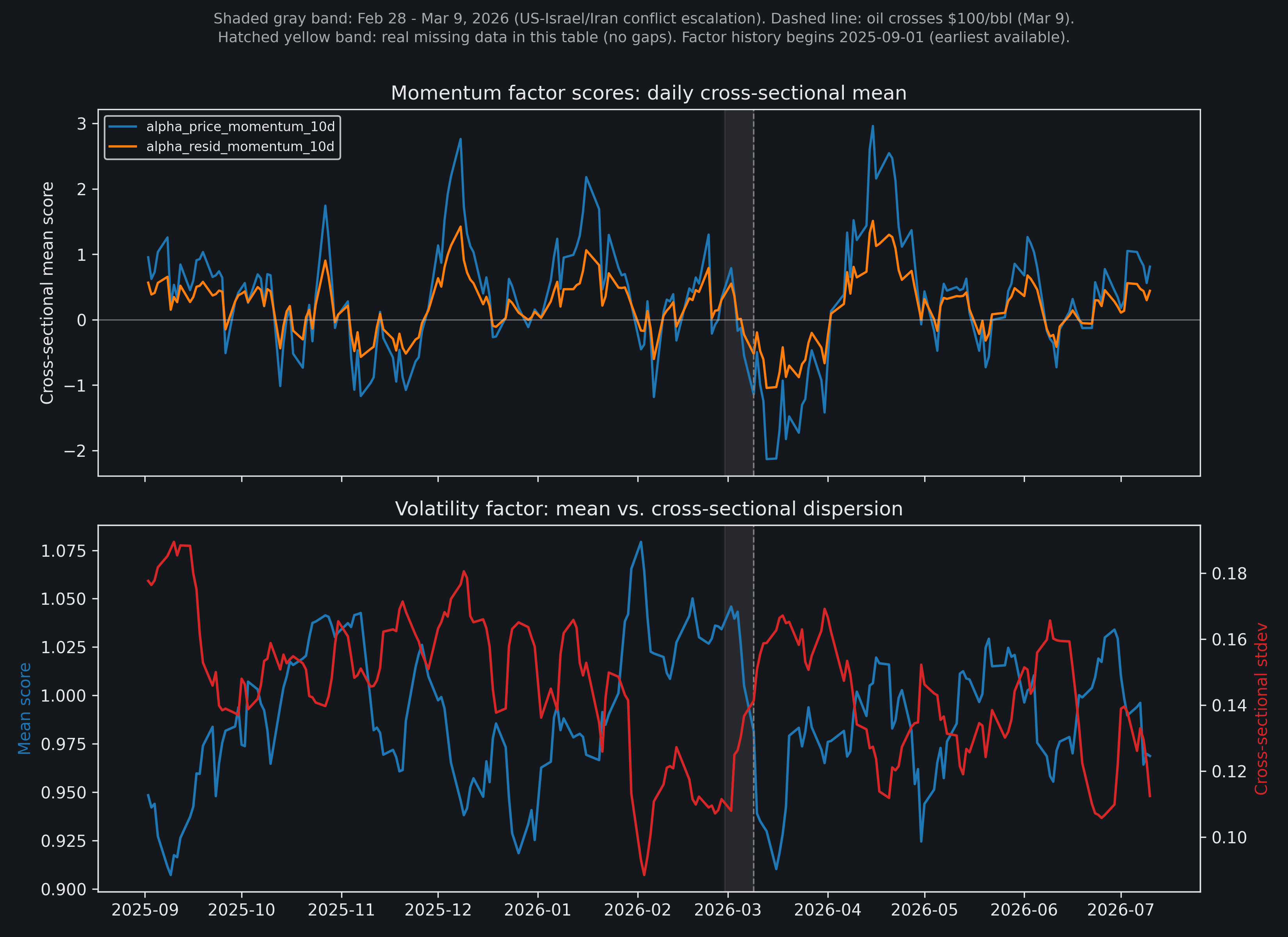
The price-momentum mean rose from 0.33 on February 27 to 0.79 on March 2, turned negative on March 4, and reached -1.14 on March 9. It continued to -2.13 on March 13, the lowest observation in the September-to-July sample. Residual momentum followed the same timing, moving from 0.30 on February 27 to -0.52 on March 9 and -1.04 on March 13, also its sample low. The trailing 10-day construction places both troughs after the defined event window.
The mean volatility score declined from 1.034 on February 27 to 0.982 on March 9. Its cross-sectional standard deviation rose from 0.112 to 0.141, an increase of about 27%. Volatility scores therefore became more dispersed across the equity universe during the window. These statistics describe the distribution of signal values; factor-portfolio returns require a separate long-short backtest.
Energy and defense prices
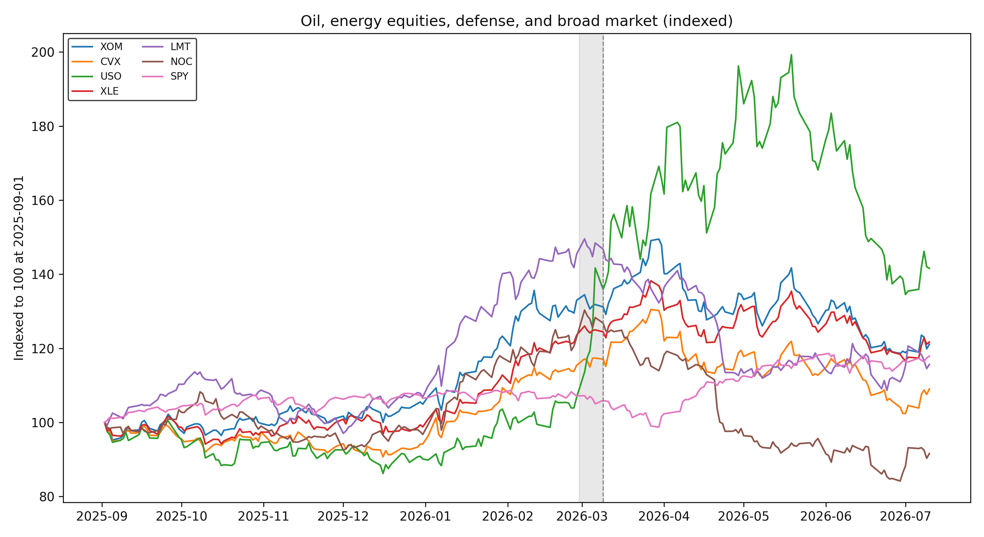
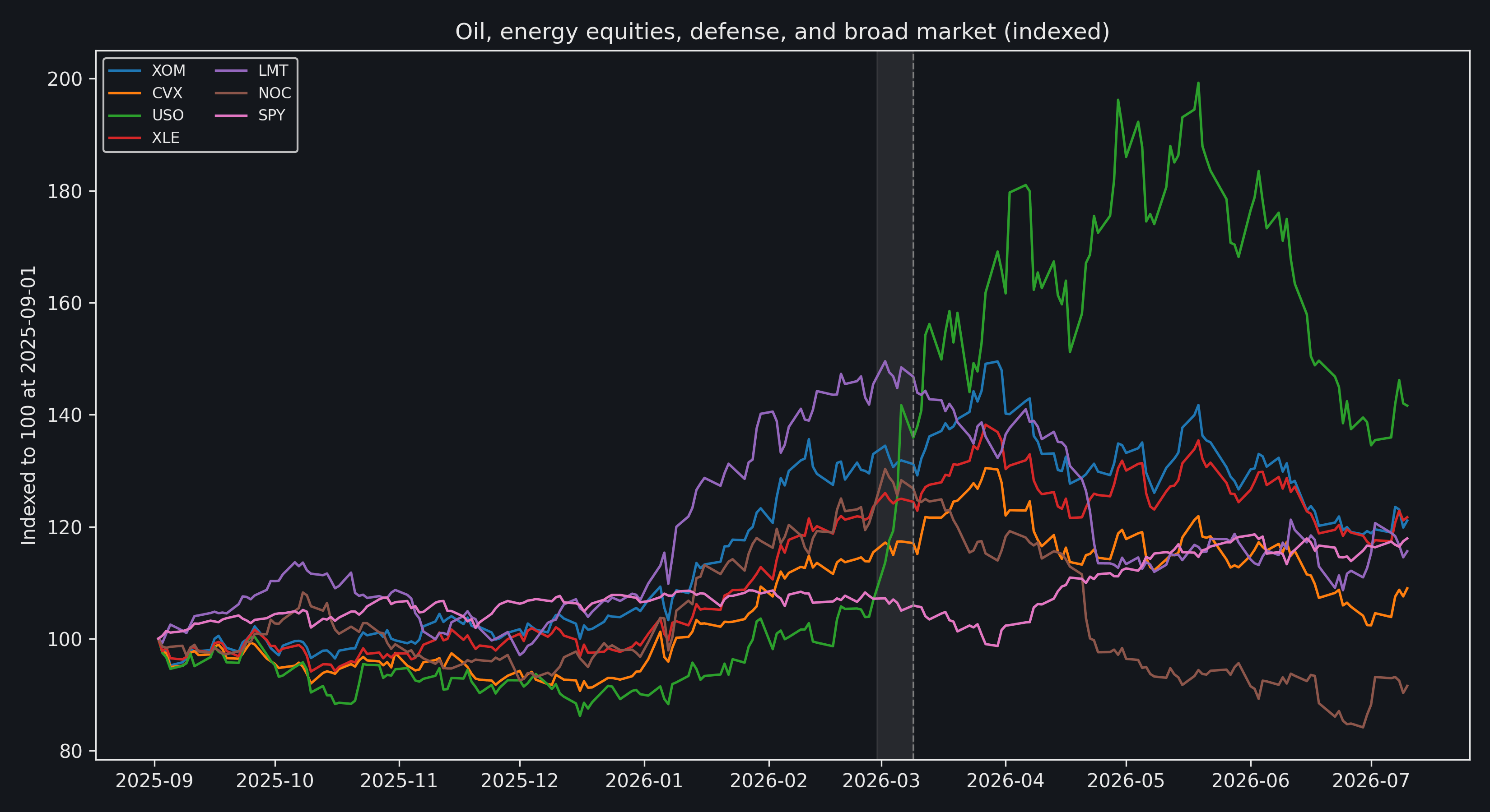
USO reached 199.3 on May 19 and ended at 141.6 on July 10. The integrated majors peaked earlier: XOM reached a maximum gain of 49.5% on March 30 and finished the sample up 21.1%; CVX reached 30.5% on March 27 and finished up 9.0%. XLE ended up 21.7% from the September baseline.
The two defense equities also followed different paths. LMT peaked 49.6% above its September level on March 2 and ended up 15.6%. NOC peaked 30.3% above the baseline on the same day and ended down 8.4%.
Refiners and integrated majors
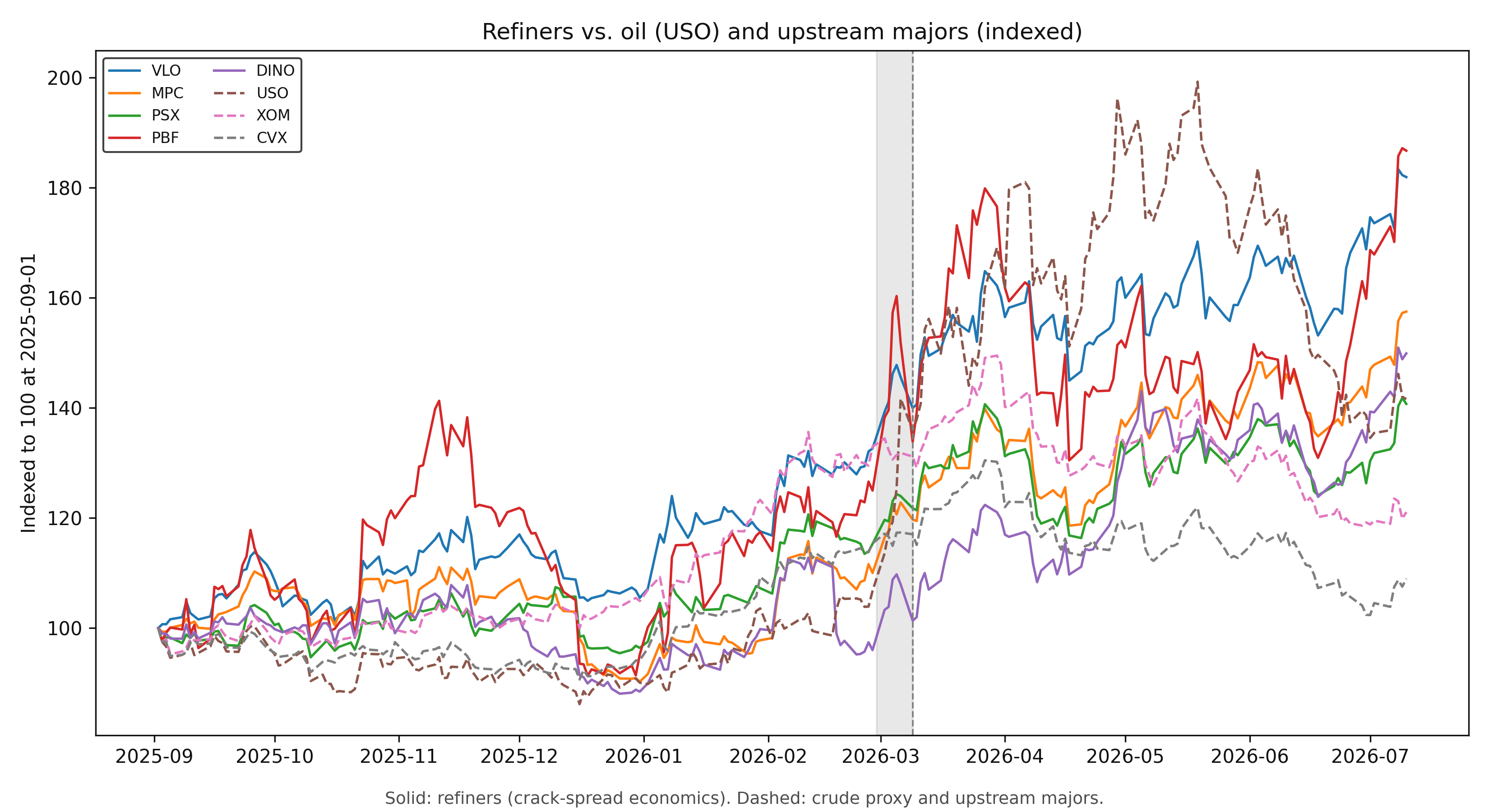
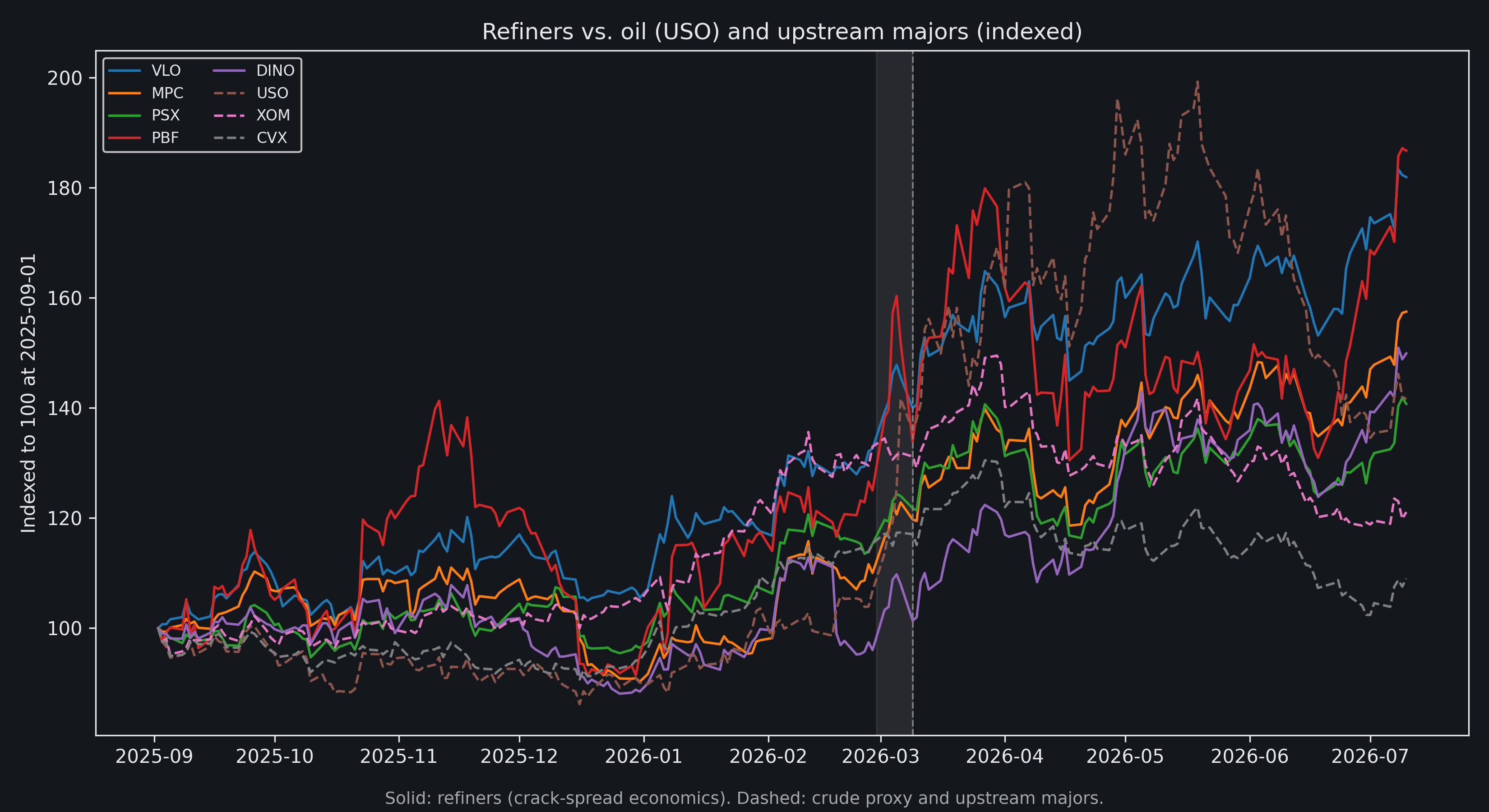
By July 10, VLO was up 81.9%, PBF 86.7%, MPC 57.5%, DINO 49.9%, and PSX 40.7%. XOM and CVX were up 21.1% and 9.0%. Product prices, crack spreads, and company earnings are needed to explain the divergence; the close series report its timing and size.
Energy-complex prices and correlations
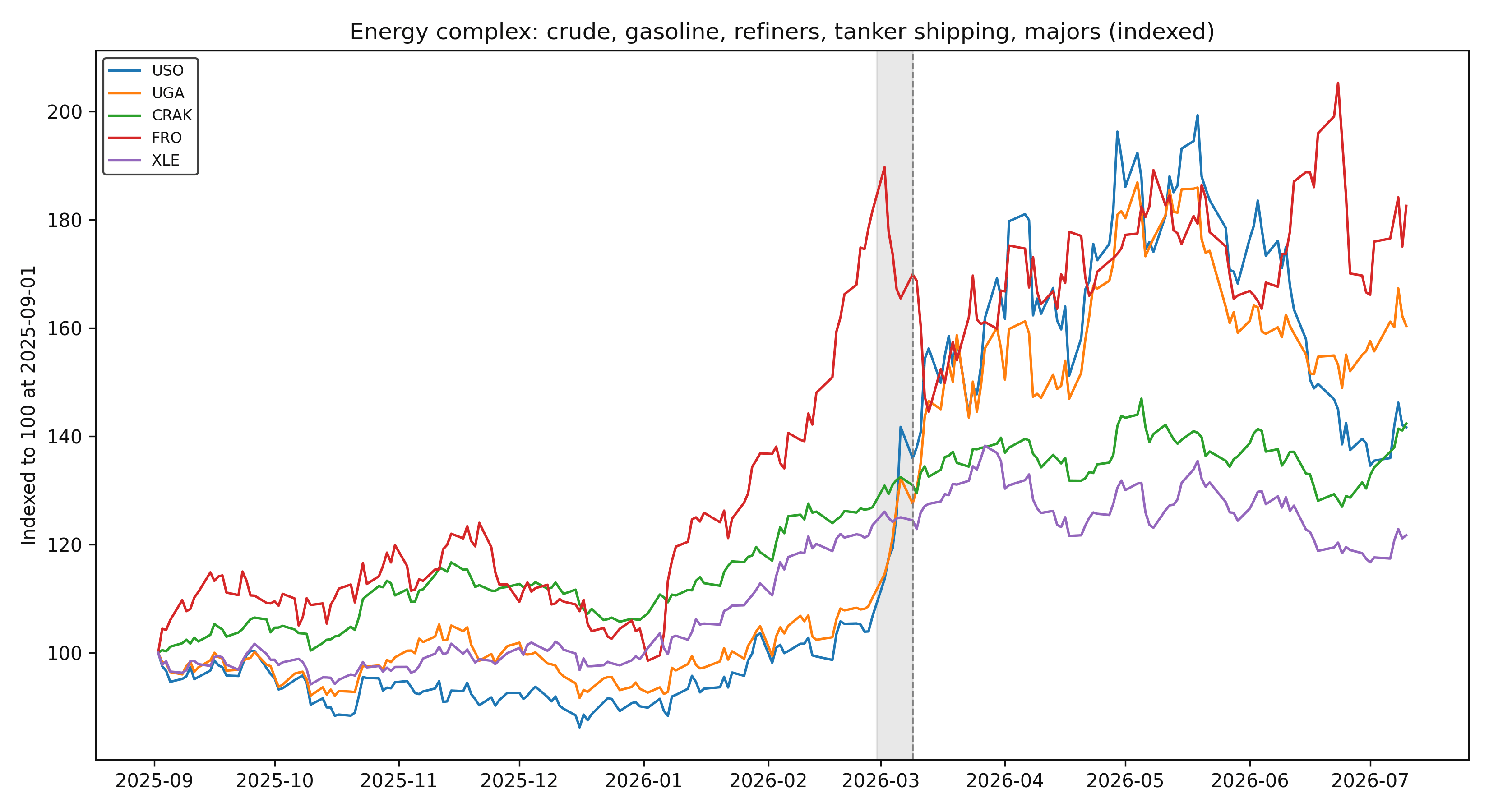
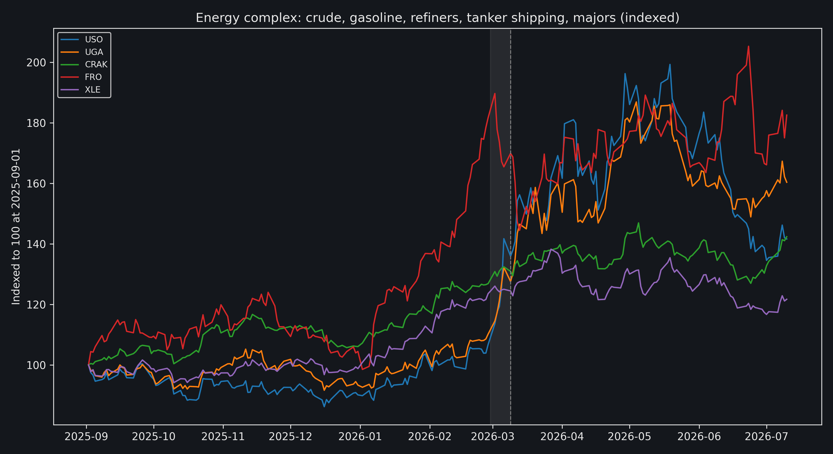
FRO had already gained 81.7% from September by February 27. It reached 189.7 on March 2, fell to 144.5 by March 13, and ended at 182.5 on July 10. An investor entering at the February 27 close experienced a 20.5% loss through March 13 and a 0.5% gain through July 10. The September-indexed return mainly preceded the hypothetical trade.
UGA ended the full sample up 60.3%, CRAK 42.3%, USO 41.6%, and XLE 21.7%. These instruments provide separate exposures to gasoline, refining margins, crude, tanker shipping, and diversified energy equities.
Pre-event correlation of daily log returns, September 2, 2025 to February 27, 2026
| Pair | Correlation |
|---|---|
| USO – UGA (crude – gasoline) | 0.89 |
| USO – XLE (crude – energy equities) | 0.74 |
| USO – CRAK (crude – refiners) | 0.45 |
| USO – FRO (crude – Frontline) | 0.21 |
| USO – BDRY (crude – dry bulk) | 0.02 |
FRO's correlations with the other energy instruments range from 0.13 to 0.22, and BDRY's from -0.04 to 0.05. These low correlations support separate tanker and dry-bulk positions. Freight rates, cargo mix, and insurance costs would be needed to refine those exposure assumptions.
Seasonality comparison
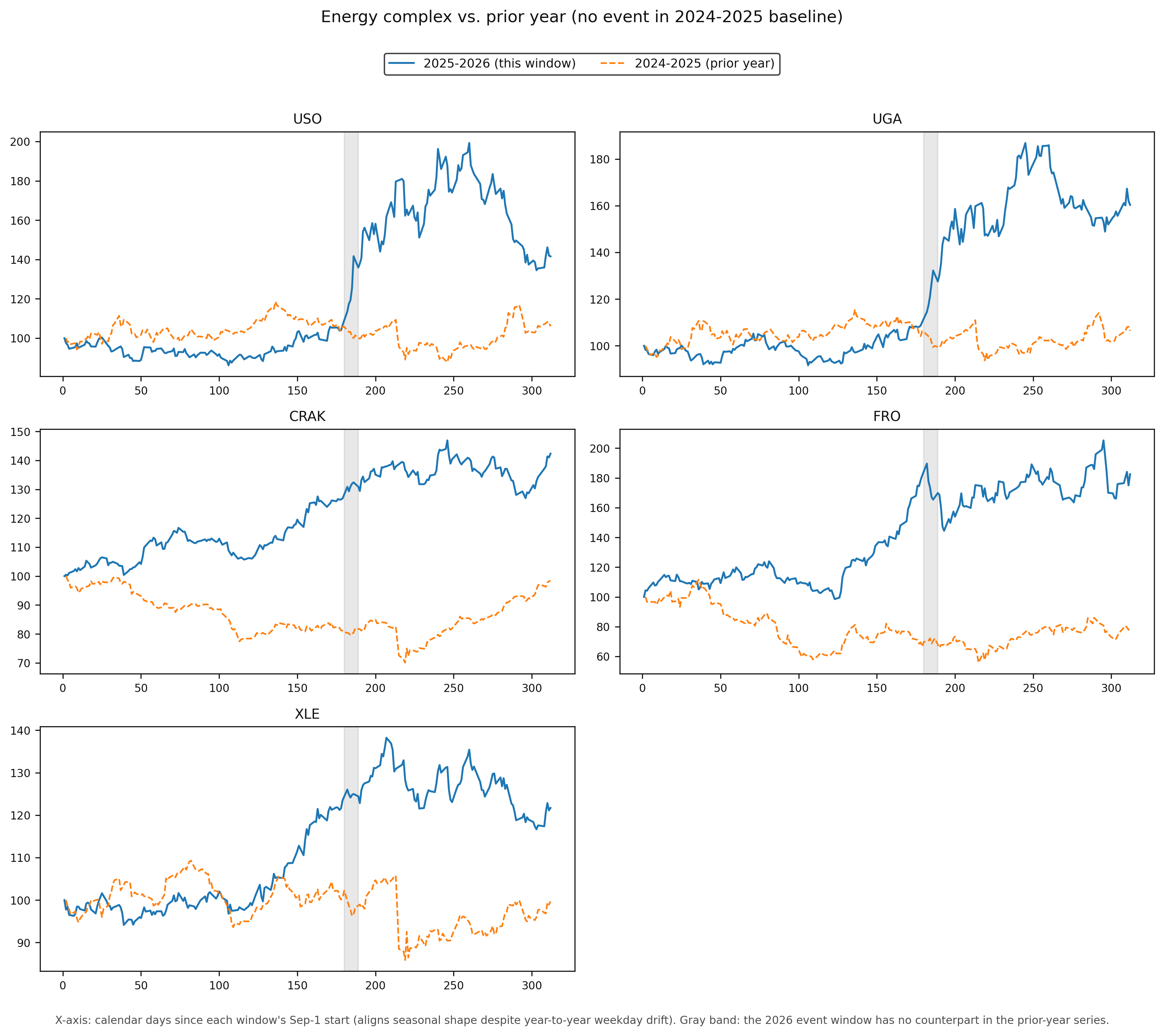
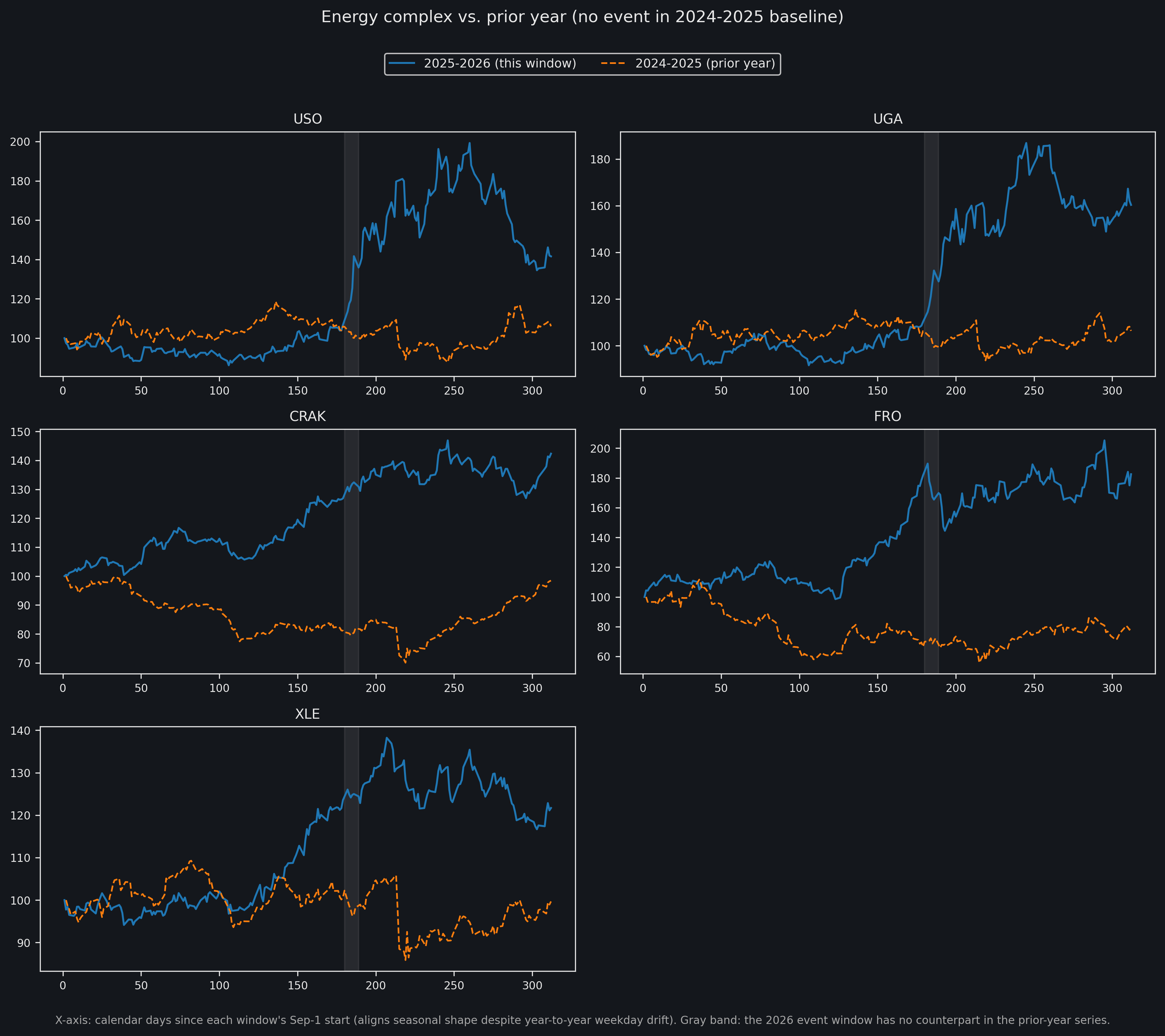
During the prior-year period, USO finished up 6.1%, UGA 6.4%, CRAK down 1.6%, FRO down 19.8%, and XLE down 0.3%. Their ranges stayed well inside the 2025-2026 moves. The current-year energy series separated sharply from their prior-year paths around the event dates.
One prior year provides a reference path. A seasonal estimate would require a longer history and controls for the other conditions that changed between the two years.
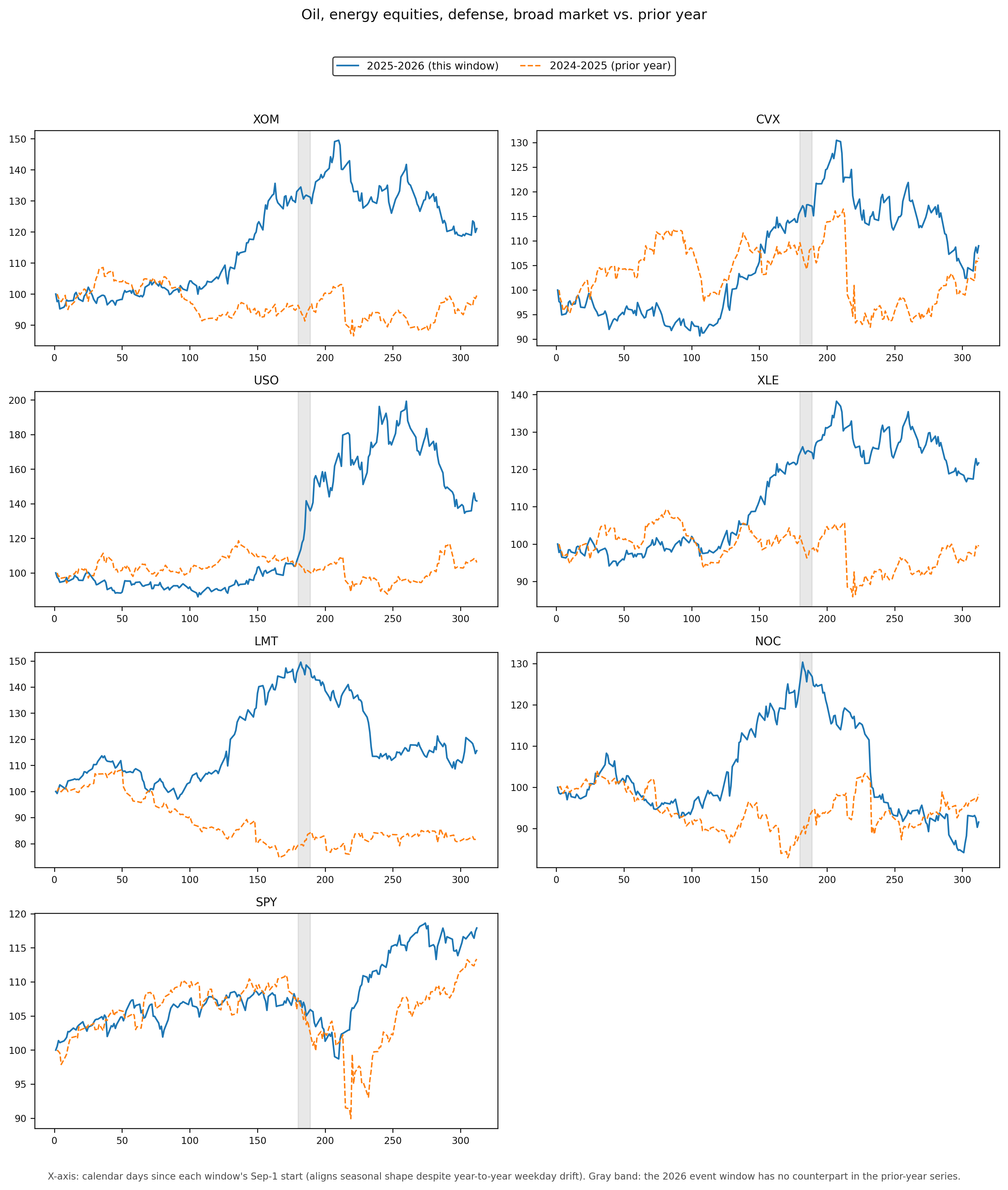
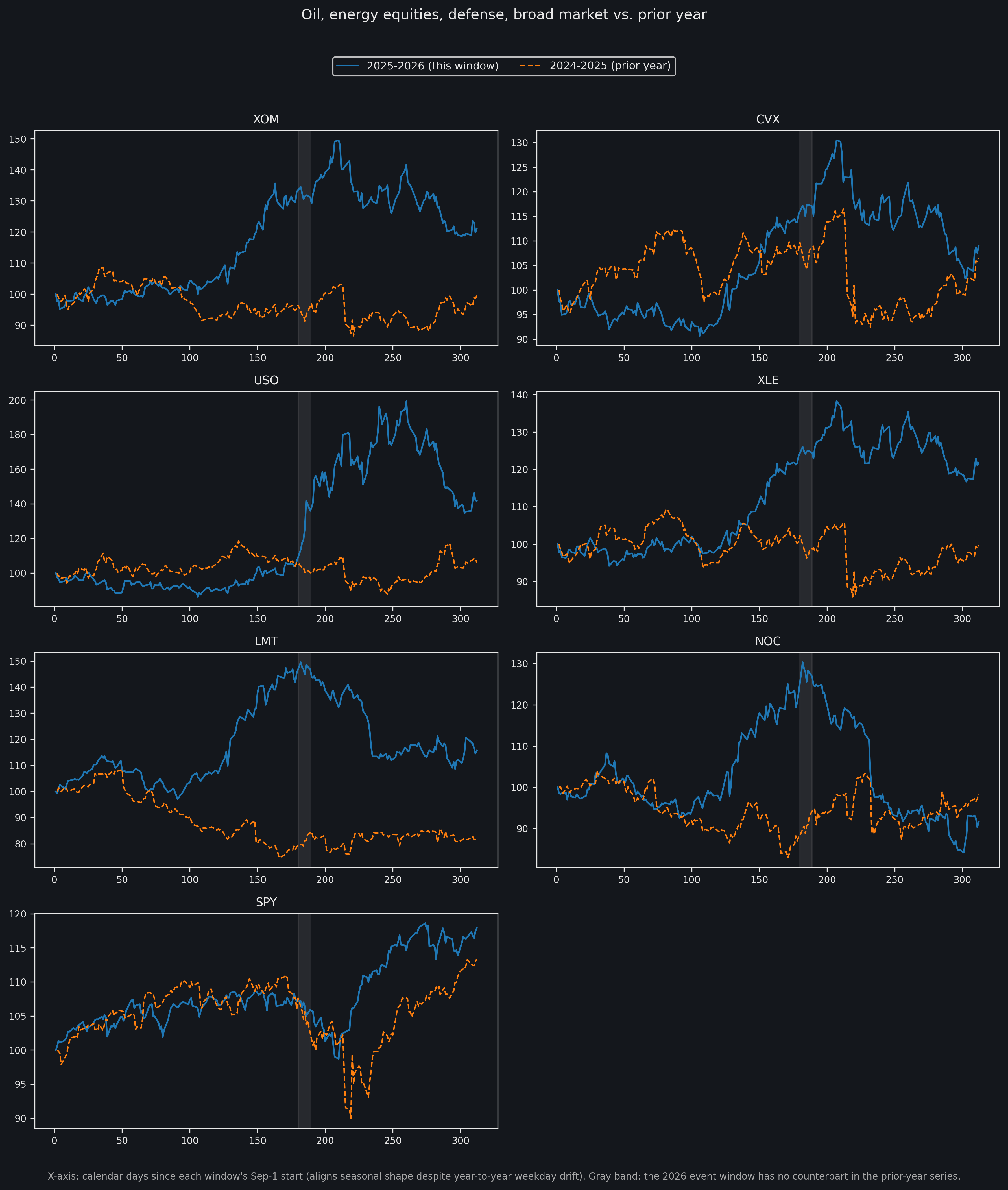
SPY's lowest level was 1.3% below its September baseline in the current window and 10.1% below the baseline in the prior-year window. The large current-year moves were concentrated in the energy and defense instruments while the broad-market path remained comparatively stable.
Sector returns
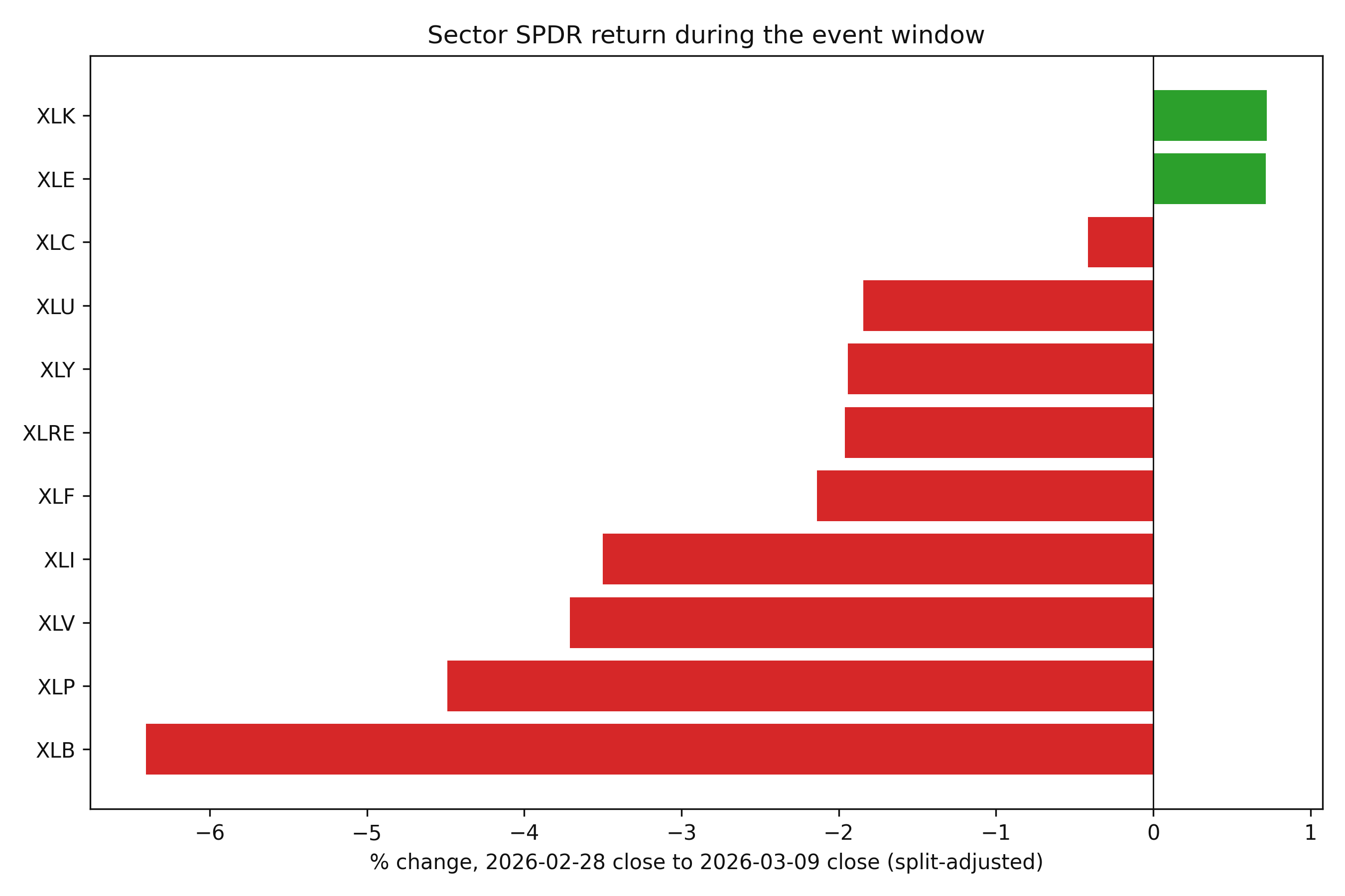
Sector SPDR price returns, February 27 close to March 9 close
| Sector ETF | Price return |
|---|---|
| XLB (Materials) | -6.40% |
| XLP (Consumer Staples) | -4.49% |
| XLV (Health Care) | -3.71% |
| XLI (Industrials) | -3.50% |
| XLF (Financials) | -2.14% |
| XLRE (Real Estate) | -1.96% |
| XLY (Consumer Discretionary) | -1.94% |
| XLU (Utilities) | -1.84% |
| XLC (Communication Services) | -0.42% |
| XLE (Energy) | +0.72% |
| XLK (Technology) | +0.72% |
Nine sector ETFs declined. Materials had the largest loss at 6.40%, followed by consumer staples at 4.49% and health care at 3.71%. Energy and technology each gained about 0.72%. Utilities lost 1.84% and ranked eighth of the eleven sectors.
Prediction-market prices
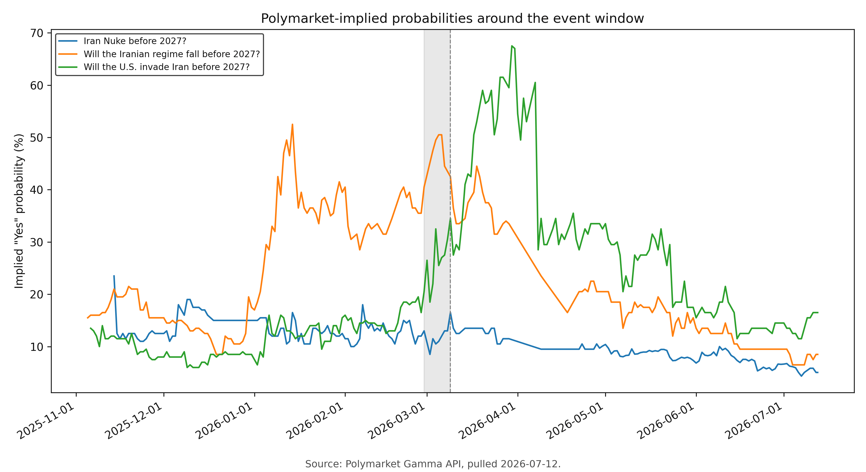
Three contracts were selected from a 40-market search because they had history before February 28 and addressed distinct outcomes: a US invasion, regime change, and an Iranian nuclear test. The chart treats the last-traded Yes price as an implied probability. A fuller probability estimate would also use market depth and bid-ask spreads.
The invasion contract rose from 19.5% on February 27 to 30.5% on March 9 and peaked at 67.5% on March 30. It ended at 16.5% on July 10. The regime-change contract moved from 35.5% to 43.5% over the event window and ended at 8.5%; its 52.5% sample high occurred on January 14. The nuclear-test contract moved from 12.0% to 13.0% during the event window.
Intraday pricing at the US open
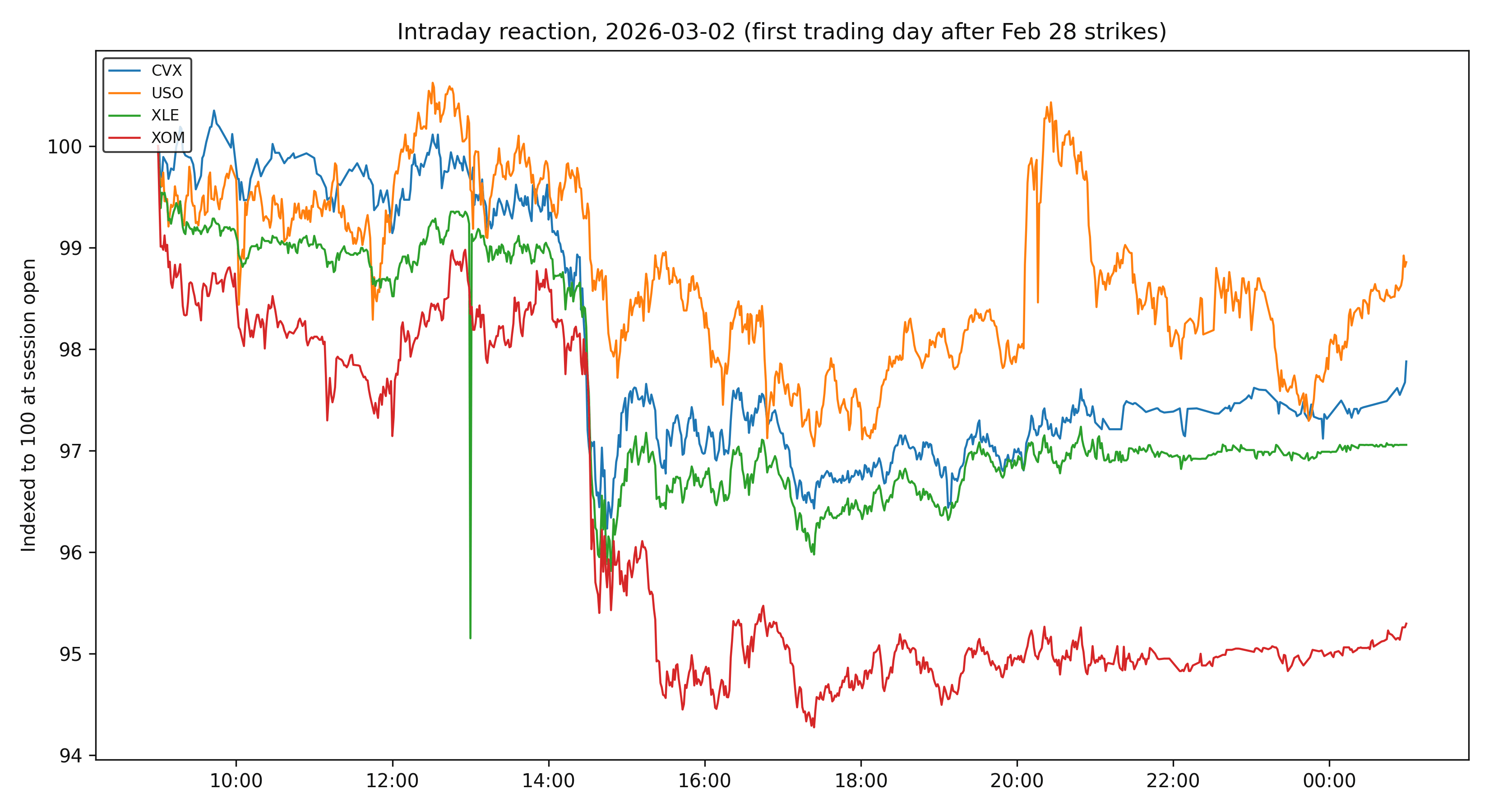
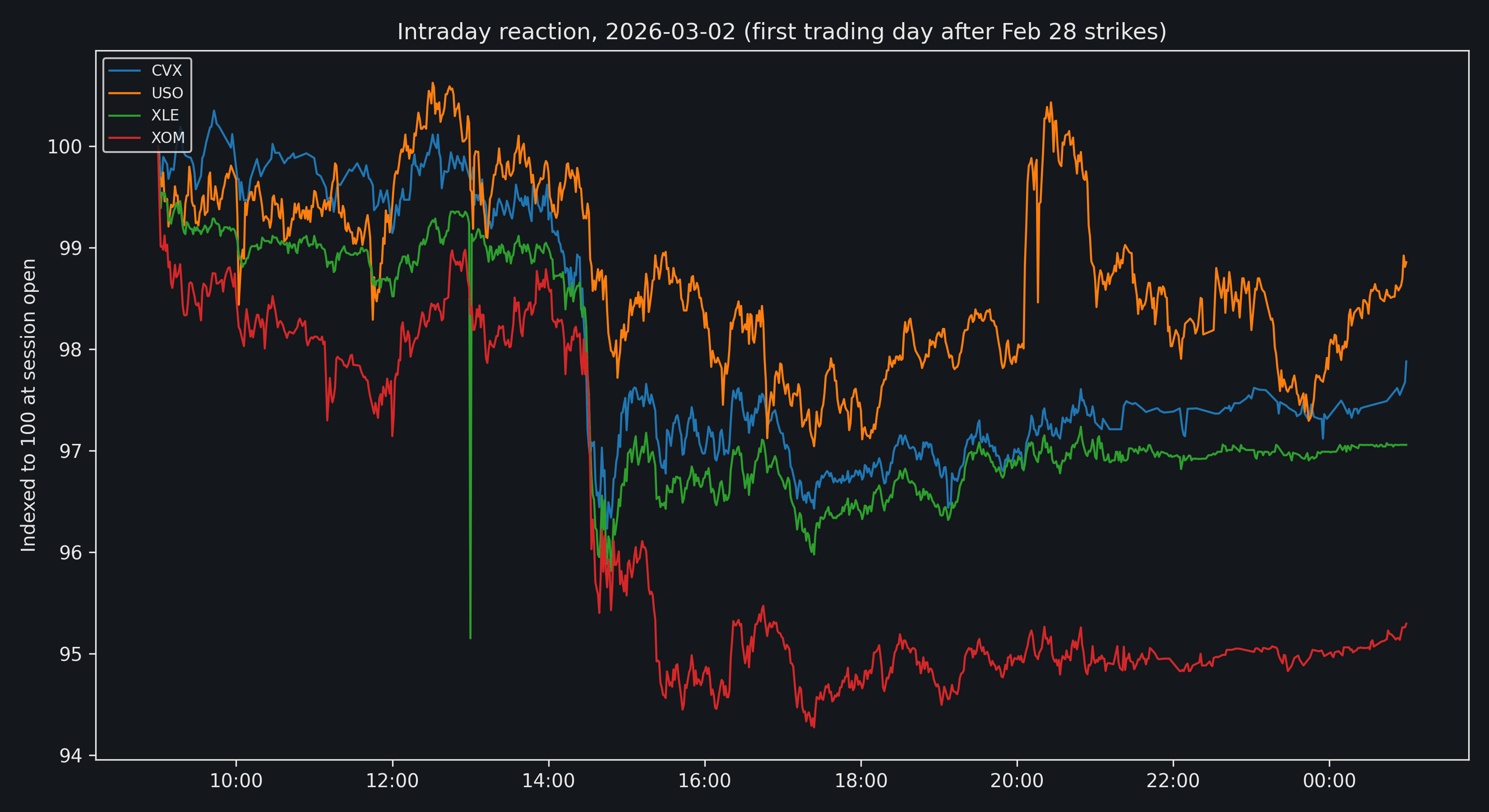
CVX, USO, XLE, and XOM all moved lower during the opening minutes of the regular session. XOM recorded the largest adjustment and traded around 97 on the normalized scale by the close. CVX recovered to approximately 100, while USO and XLE finished near 99. Attribution would require contemporaneous news and order-flow records.
Probability-weighted portfolio construction
Set the decision time at the February 27 close and the forecast horizon at ten trading sessions, ending March 13. The conditional event view assigns the largest returns to crude and gasoline, followed by Frontline, refiners, and diversified energy equities. View construction ends at the decision time; prices after February 27 are reserved for evaluation.
Conditional 10-session view and subsequent split-adjusted price returns
| Asset | Conditional view | March 13 | July 10 |
|---|---|---|---|
| USO | +6.0% | +46.3% | +32.6% |
| UGA | +5.0% | +32.9% | +45.5% |
| FRO | +3.0% | -20.5% | +0.5% |
| CRAK | +2.5% | +4.4% | +12.2% |
| XLE | +2.0% | +3.2% | -1.5% |
| Cash | +0.1% | +0.1% | +1.3% |
USO and UGA exceeded the conditional return assumptions. CRAK and XLE gained less, while FRO fell. By July, UGA had the largest return from the decision date, FRO was approximately flat, and XLE was lower.
The covariance matrix uses split-adjusted daily log returns from September 2 through February 27 and is scaled to ten sessions. Cash uses the 3.67% coupon-equivalent 13-week Treasury bill rate on February 27. The portfolio is long-only and fully funded, with a risk-aversion coefficient of 30. Trading costs, taxes, distributions, and rebalancing are set to zero.
Let \(v\) denote the conditional excess-return vector and \(p\) the probability assigned to the event view. The baseline state assigns each risky asset the cash return. Expected return and covariance for each run are
\[\mu(p) = r_f\mathbf{1} + p v,\]
\[\Sigma(p) = \Sigma_{\mathrm{pre}} + p(1-p)vv^\top.\]
The second term records the variance between the event and baseline outcomes. The model applies the pre-event covariance estimate in both states. The 85%, 50%, and 25% probabilities are sensitivity inputs. The Polymarket contracts above address different outcomes; translating their prices into a supply-disruption probability would require an additional mapping. The optimizer solves
\[\max_{w \ge 0} \left[ \mu(p)^\top w - \frac{\lambda}{2}w^\top\Sigma(p)w \right] \quad\text{subject to}\quad \mathbf{1}^\top w = 1.\]
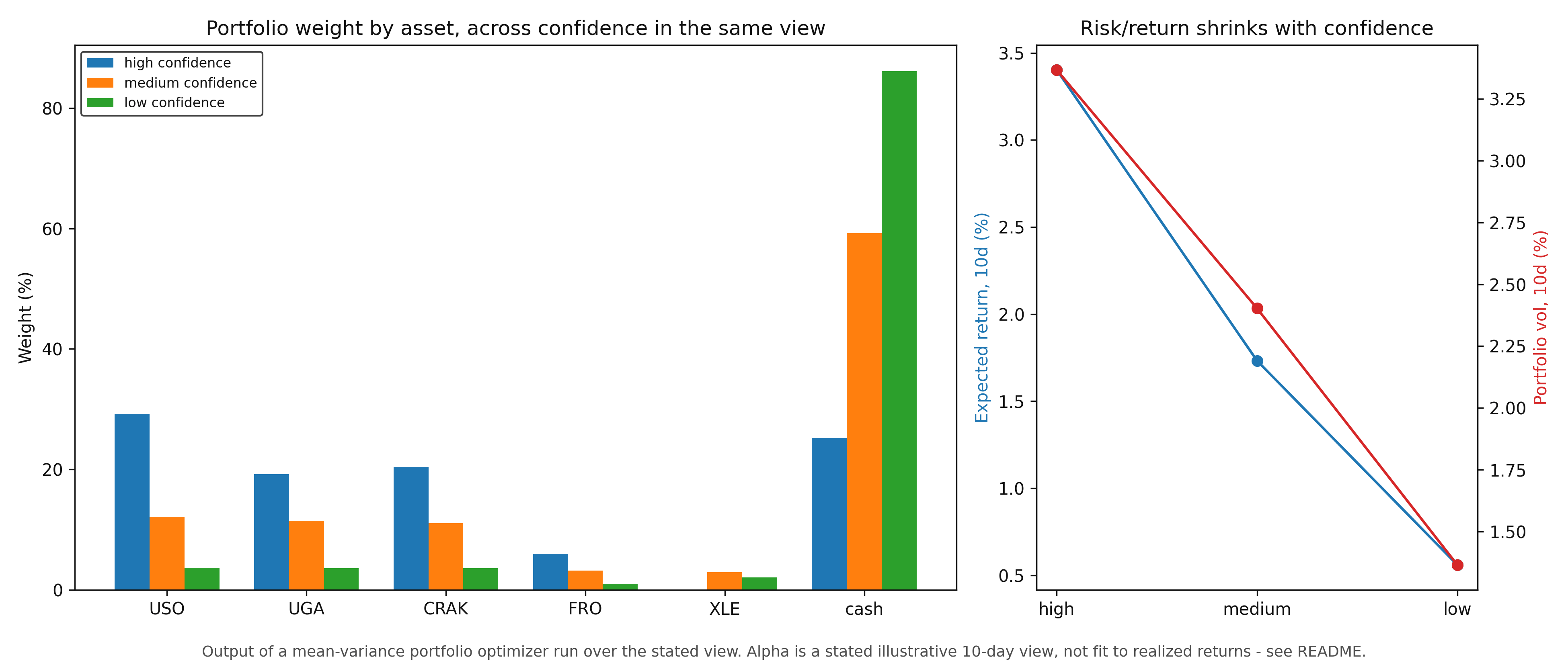
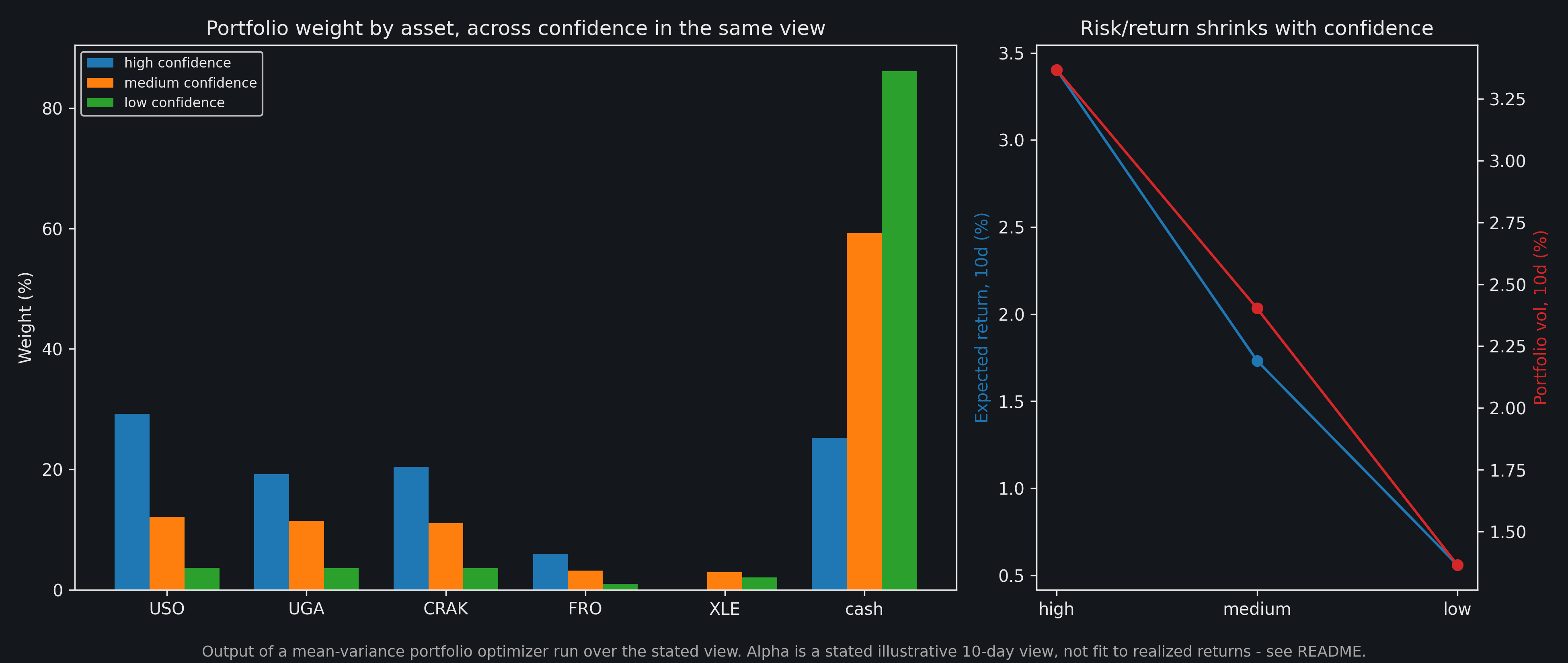
At 85%, the optimizer assigns 40.3% to USO, 14.7% to CRAK, 4.7% to FRO, and 40.1% to cash. UGA receives 0.2% because its 0.89 pre-event correlation with USO makes the higher-return USO forecast dominant in this setup. XLE receives zero. At 50%, cash rises to 68.6%; at 25%, it rises to 83.4%. The relative proportions of USO, CRAK, and FRO remain similar as total capital committed to the view declines.
Forecast portfolio statistics and subsequent buy-and-hold returns
| Configuration | Cash | Expected 10d return | Expected 10d vol | March 13 | July 10 |
|---|---|---|---|---|---|
| View probability 85% | 40.1% | 2.6% | 2.8% | +18.4% | +15.6% |
| View probability 50% | 68.6% | 0.9% | 1.6% | +9.7% | +8.8% |
| View probability 25% | 83.4% | 0.3% | 0.8% | +5.2% | +5.3% |
| All cash | 100% | 0.1% | 0.0% | +0.1% | +1.3% |
| 100% USO | 0% | 6.0% | 5.6% | +46.3% | +32.6% |
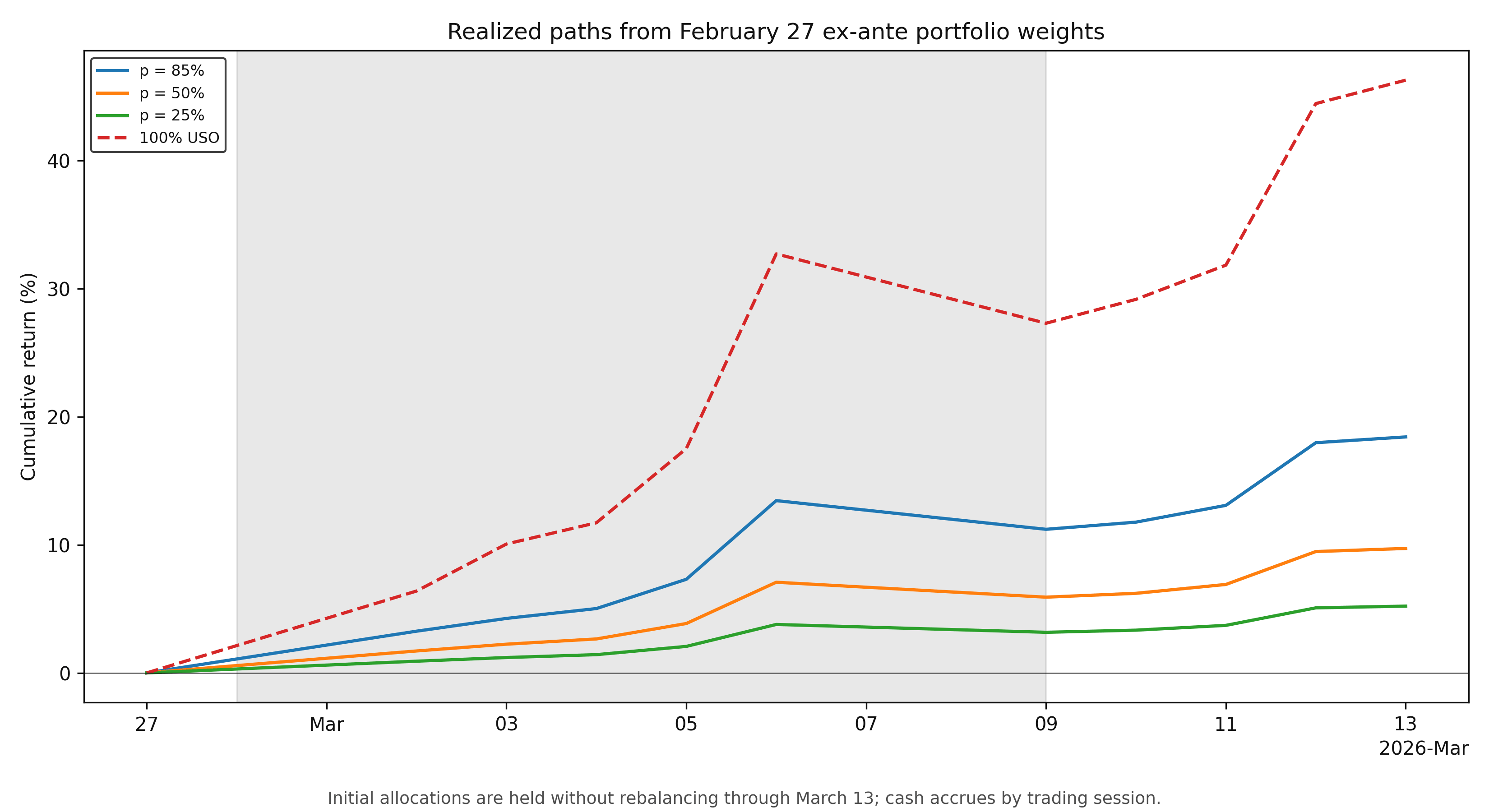
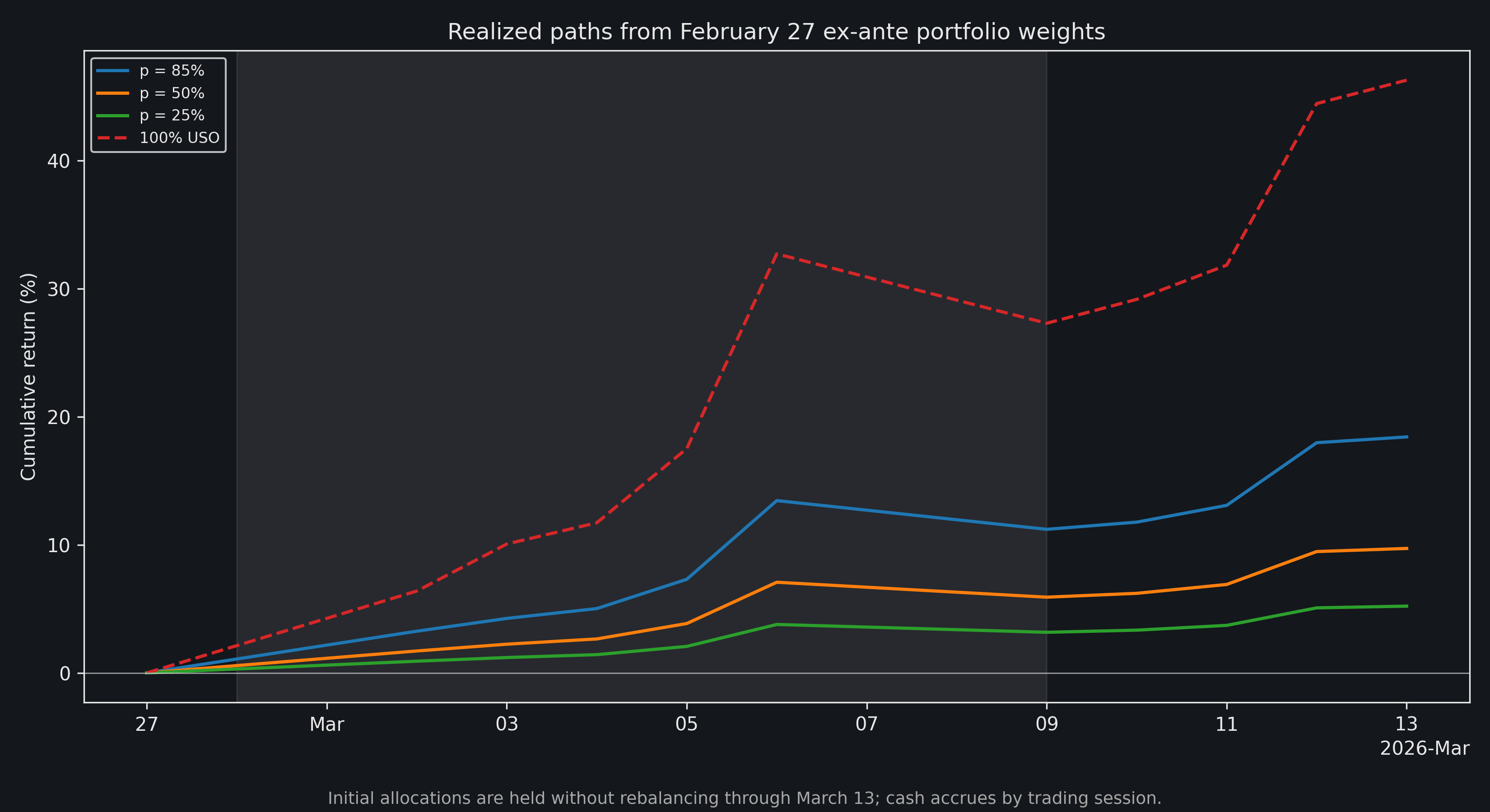
The February 27 weights remain fixed through March 13. Each line therefore evaluates the original decision-date allocation at subsequent closing prices.
The full-view, concentrated USO benchmark earned the highest subsequent return and carried twice the forecast volatility of the 85% portfolio. The probability-weighted portfolios committed less capital and spread the risky position across three instruments. FRO detracted during the first ten sessions, while CRAK contributed positively over both evaluation dates.
This walkthrough is for research and educational purposes. It illustrates how strategynet.ai organizes signal evidence into factors and scenarios. It provides no recommendation, investment advice, or instruction to trade any security.
Back to Insights