
What Is Factor Crowding?
Factor crowding is the concentration of capital in similar investment positions. It matters because shared holdings can lead to correlated selling when investors reduce exposure, increasing losses and demands on liquidity. Researchers estimate crowding from ownership, positioning, trading, liquidity, and return data.
This article develops a short-crowding factor from observable inputs. It follows the calculation through normalization, a five-stock example, predictive evaluation, and portfolio construction, showing how a crowding hypothesis becomes a testable investment signal.
From the idea to a measurable definition
Suppose the research question is:
Among otherwise eligible US equities, which names show the greatest short-crowding pressure and therefore the greatest potential for a squeeze or disorderly covering?
Three measurements can represent different parts of that question:
- Days to cover relates open short positions to ordinary trading capacity.
- Short-sale volume ratio measures recent short-selling flow in the reported venue data.
- Recent return indicates whether price action has already moved against the short side.
For security \(i\) at observation time \(t\), define days to cover as
\[DTC_{i,t} = \frac{SI_{i,t^*}} {\frac{1}{L}\sum_{\ell=1}^{L}V_{i,t-\ell}},\]
where \(SI_{i,t^*}\) is the latest short-interest position that was publicly available by \(t\), \(V\) is daily share volume, and \(L\) is the average-volume window. The date \(t^*\) may precede \(t\) because short-interest reports are periodic. A point-in-time test uses the report that was actually available at the decision time, including its publication lag.
For a clearly identified set of reporting venues, the daily short-sale volume ratio is
\[SVR_{i,t} = \frac{SSV_{i,t}}{RV_{i,t}},\]
where \(SSV\) is reported short-sale volume and \(RV\) is the corresponding reported total volume. This is a flow measure. It is not the proportion of a company's shares currently held short, and it should not be described as short interest.
Let the recent price component be the close-to-close return over \(H\) trading days:
\[r^{(H)}_{i,t} = \frac{P_{i,t}}{P_{i,t-H}}-1.\]
These three quantities now have dates and units, but they still cannot be added directly. Days, percentages, and returns need a common cross-sectional scale.
Cross-sectional normalization
For a transparent hand calculation, use a centred percentile rank. If \(\operatorname{rank}_{U_t}(x_{i,t})\) assigns 1 to the smallest value and \(N_t\) to the largest value among the eligible securities \(U_t\), define
\[q(x_{i,t}) = 2\left( \frac{\operatorname{rank}_{U_t}(x_{i,t})-1}{N_t-1} \right)-1.\]
The transformation maps the lowest observation to \(-1\), the middle of an odd cross-section to \(0\), and the highest observation to \(+1\). A production definition also states the tie method, minimum coverage, missing-value rule, and any winsorization applied before ranking. A winsorized z-score is another valid choice, but it will not produce the same distances between securities.
One possible short-crowding score is
\[C_{i,t} = 0.40q(DTC_{i,t}) +0.35q(SVR_{i,t}) -0.25q(r^{(5)}_{i,t}).\]
The negative sign on recent return is deliberate. In this definition, high days to cover, high short-selling flow, and weak recent price performance raise the score. The weights express a research choice and belong to the versioned factor definition. A study of short-covering already under way might instead give recent positive returns a positive sign. Both are coherent questions, but they are different factors.
Worked five-stock example
Assume the following values were available at the observation cutoff. Short interest and average daily volume are shown only to make the days-to-cover calculation visible. The company labels and values are illustrative.
Point-in-time inputs for the crowding example
| Security | Short interest | 20-day ADV | Days to cover | Short-volume ratio | 5-day return |
|---|---|---|---|---|---|
| A | 20.0m | 2.0m | 10.0 | 45% | −2% |
| B | 12.0m | 2.0m | 6.0 | 60% | +4% |
| C | 6.0m | 2.0m | 3.0 | 30% | −8% |
| D | 4.0m | 2.0m | 2.0 | 20% | +1% |
| E | 2.0m | 2.0m | 1.0 | 10% | +8% |
Security A has \(20/2=10\) days to cover. Across these five names, A has the highest days-to-cover rank, the second-highest short-volume rank, and the second-weakest recent return. Its centred ranks are therefore \(+1.00\), \(+0.50\), and \(-0.50\). Substitution into the score gives
\[C_{A,t} =0.40(1.00)+0.35(0.50)-0.25(-0.50) =0.700.\]
Applying the same calculation to the complete cross-section gives:
Normalized components and composite crowding score
| Security | q(DTC) | q(SVR) | q(5-day return) | Crowding score |
|---|---|---|---|---|
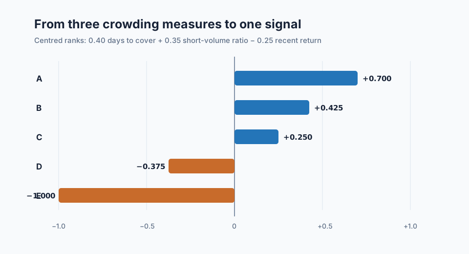
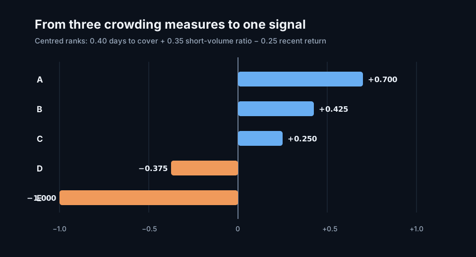
| A | +1.00 | +0.50 | −0.50 | +0.700 |
| B | +0.50 | +1.00 | +0.50 | +0.425 |
| C | 0.00 | 0.00 | −1.00 | +0.250 |
| D | −0.50 | −0.50 | 0.00 | −0.375 |
| E | −1.00 | −1.00 | +1.00 | −1.000 |
B and C demonstrate why the composite is useful. B has the highest short-sale flow but has already risen, while C has only middle-ranked positioning proxies and a very weak recent return. Their final scores are close for different reasons, which remains visible in the component record.
Python calculation
import pandas as pd

observations = pd.DataFrame(
    {
        "days_to_cover": [10.0, 6.0, 3.0, 2.0, 1.0],
        "short_volume_ratio": [0.45, 0.60, 0.30, 0.20, 0.10],
        "return_5d": [-0.02, 0.04, -0.08, 0.01, 0.08],
    },
    index=["A", "B", "C", "D", "E"],
)

def centred_rank(series):
    percentile = (series.rank(method="average") - 1) / (series.count() - 1)
    return 2 * percentile - 1

ranked = observations.apply(centred_rank)
score = (
    0.40 * ranked["days_to_cover"]
    + 0.35 * ranked["short_volume_ratio"]
    - 0.25 * ranked["return_5d"]
)

print(score.round(3))
The code assumes complete coverage and no ties. Those assumptions are helpful for this example and unsuitable as silent production defaults.
When the score becomes a factor
The score \(C_{i,t}\) is the security-level signal observed for one security on one date. The factor is the repeatable, versioned rule that produces the whole cross-section \(\mathbf{C}_t=(C_{1,t},\ldots,C_{N_t,t})\) at every scheduled observation time. Its definition includes the data sources, availability lag, eligible universe, transformations, weights, orientation, calculation cutoff, and forecast horizon.
The implementation records each dated output as a signal observation linked to its factor definition. A factor-mimicking portfolio adds the holdings that represent the factor in returns. These links allow researchers to trace a portfolio result back to the scores and calculation that produced it.
The factor is tested against a stated outcome. For a squeeze-pressure study, one could measure the cross-sectional information coefficient between \(C_{i,t}\) and each security's return from \(t+1\) through \(t+h\):
\[IC_t = \operatorname{corr}_{i\in U_t} \left( \operatorname{rank}(C_{i,t}), \operatorname{rank}(R_{i,t+1:t+h}) \right).\]
A positive IC means higher crowding scores tended to precede higher returns at that horizon. A negative IC means they tended to precede lower returns. Either result can be economically informative, provided the intended direction was declared before examining the test period.
From factor scores to portfolio weights
A simple demonstration converts the centred scores directly into a dollar-neutral, unit-gross vector:
\[w_{i,t}^{\mathrm{simple}} = \frac{C_{i,t}}{\sum_{j\in U_t}|C_{j,t}|}.\]
The five example scores sum to zero and have absolute sum \(2.75\), producing weights of approximately \(+25.5\%\), \(+15.5\%\), \(+9.1\%\), \(-13.6\%\), and \(-36.4\%\). This arithmetic shows the conversion, but it ignores covariance, liquidity, sectors, size, and position limits.
A pure factor-mimicking portfolio instead chooses weights with exposure to the crowding score while controlling other risks. One form is
\[\begin{aligned} \min_{\mathbf{w}_t}\quad & \frac{1}{2}\mathbf{w}_t^\top\Sigma_t\mathbf{w}_t \\ \text{subject to}\quad & \mathbf{w}_t^\top\mathbf{C}_t=1, \\ & \mathbf{w}_t^\top\mathbf{1}=0, \\ & \mathbf{w}_t^\top B_t=\mathbf{0}, \\ & |w_{i,t}|\leq \ell_i. \end{aligned}\]
\(\Sigma_t\) is the point-in-time covariance estimate, \(B_t\) contains unwanted exposures such as sectors and size, and \(\ell_i\) sets position limits. The resulting return series shows how the selected crowding definition behaved after those common exposures were constrained. It remains a research result; combining it with other validated factors and client constraints is a separate portfolio decision.
Positive, zero, and negative crowding scores
A positive value indicates above-centre crowding pressure under this exact orientation. Zero places a security near the cross-sectional balance of the three weighted components, or records offsetting positive and negative components. A negative value indicates below-centre pressure.
The sign does not say whether the security should be bought or sold without a forecast question. A high score could support a tactical long squeeze study, a risk limit on an existing short, or an exclusion from a portfolio whose exit liquidity is already fragile. The same measurement can inform several decisions without making them equivalent.
Other forms of crowding
Short-position data covers only one part of the subject. Long-side crowding may be studied using institutional ownership, fund holdings, securities-lending conditions, valuation spreads, or common changes in positions. Return-based measures such as comomentum infer common trading from abnormal correlation among securities held by a strategy. Each proxy has its own frequency, coverage, and delay.
Crowding can also be measured at the factor or portfolio level. If many strategies hold similar value, momentum, quality, or volatility positions, the relevant object may be common factor exposure rather than one company's short position. The research definition should match that level.
Common implementation mistakes
Treating short-sale volume as short interest
Short-sale volume counts reported transactions during a period. Short interest is a snapshot of open short positions. A short sale opened and closed on the same day can appear in volume without appearing in the next short-interest snapshot, while an older open position can remain in short interest without generating new short-sale volume that day.
Backdating a later report
The effective date printed on a short-interest record is not necessarily the date on which the data became available. Historical calculations must use the publication timestamp known to the analyst at \(t\).
Mixing venue coverage
A ratio built from off-exchange short-sale volume and consolidated total volume does not have a consistent numerator and denominator. The selected feeds and coverage should be named in the definition and kept stable through the test.
Ignoring liquidity and corporate actions
Splits affect share counts, and thin volume can make days to cover unstable. Point-in-time adjustment, liquidity eligibility, and extreme-value treatment need recorded rules.
Selecting the sign after seeing returns
Squeeze continuation and crowded-position underperformance are both plausible research questions. Reversing a score after inspecting the holdout period turns that period into training data.
Assuming purification removes every common risk
Neutralization controls exposures included in \(B_t\). It cannot remove an unmeasured common exit, stale covariance, nonlinear option exposure, or a liquidity shock that changes market relationships.
Frequently asked questions
Is a crowded factor necessarily unprofitable?
No. Crowding can coexist with a positive expected return. It changes the liquidity, correlation, and tail-risk profile, especially when many holders face similar losses or funding constraints.
Why include recent return in the example?
Positioning and flow say little about whether pressure is already resolving. Recent price action helps distinguish heavy shorts that remain comfortable from those being challenged by the market. The sign depends on the intended forecast.
Can the weights be learned from data?
Yes, provided every historical score uses coefficients estimated only from data available before that observation. Fixed weights are easier to audit; adaptive weights require a walk-forward training and versioning schedule.
Does a high crowding score prove that a squeeze will occur?
No. It orders securities by a stated set of proxies. Predictive value must be measured across later returns, and the most crowded names can remain crowded or decline further for fundamental reasons.
Next reading
- What Is a Trading Signal in Quantitative Finance?
- Alpha factor: a cross-sectional signal that ranks expected returns
- How to compose registered signals into a factor
Sources
- FINRA, “Short Interest – What It Is, What It Is Not”.
- FINRA, “Understanding Short Sale Volume Data on FINRA's Website”.
- SEC, “Key Points About Regulation SHO”.
- Dong Lou and Christopher Polk, “Comomentum: Inferring Arbitrage Activity from Return Correlations”, The Review of Financial Studies, 2022.
- Lasse Heje Pedersen, “When Everyone Runs for the Exit”, International Journal of Central Banking, 2009.
This walkthrough is for research and educational purposes. It illustrates how strategynet.ai organizes signal evidence into factors and scenarios. It provides no recommendation, investment advice, or instruction to trade any security.
Back to Insights