
How does tax-aware portfolio optimization change a rebalance?
Tax-aware portfolio optimization chooses trades and tax lots by comparing the investment benefit with implementation cost, current tax, and the value of continued tax deferral. Its objective is to improve after-tax wealth while satisfying the account's cash, exposure, and liquidity constraints.
The four hypothetical examples below follow gains, loss harvesting, wash-sale state, and tax funding through a rebalance. Each traces the proposed trade into cash, recognized gains or losses, and the remaining tax basis, showing how today's decision affects the next one. The examples use illustrative prices, forecasts, rates, and loss capacity for educational purposes.
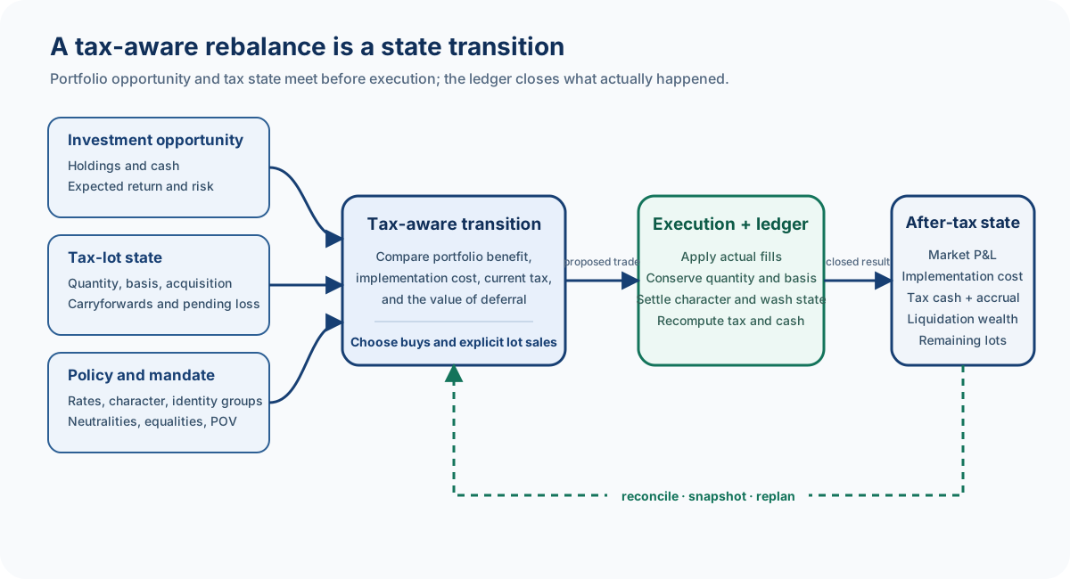
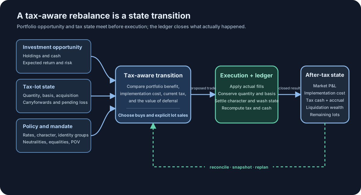
Market movement creates P&L; the sale sets recognition
Suppose a portfolio owns 2,000 shares bought for USD 60 and now worth USD 100. The position has a market value of USD 200,000, basis of USD 120,000, and an embedded gain of USD 80,000.
That USD 80,000 was earned as the price rose. Selling the position changes the gain from unrealized to realized and may create tax cash, but it does not add another USD 80,000 to investment P&L. This distinction is the starting point for a clean after-tax comparison.
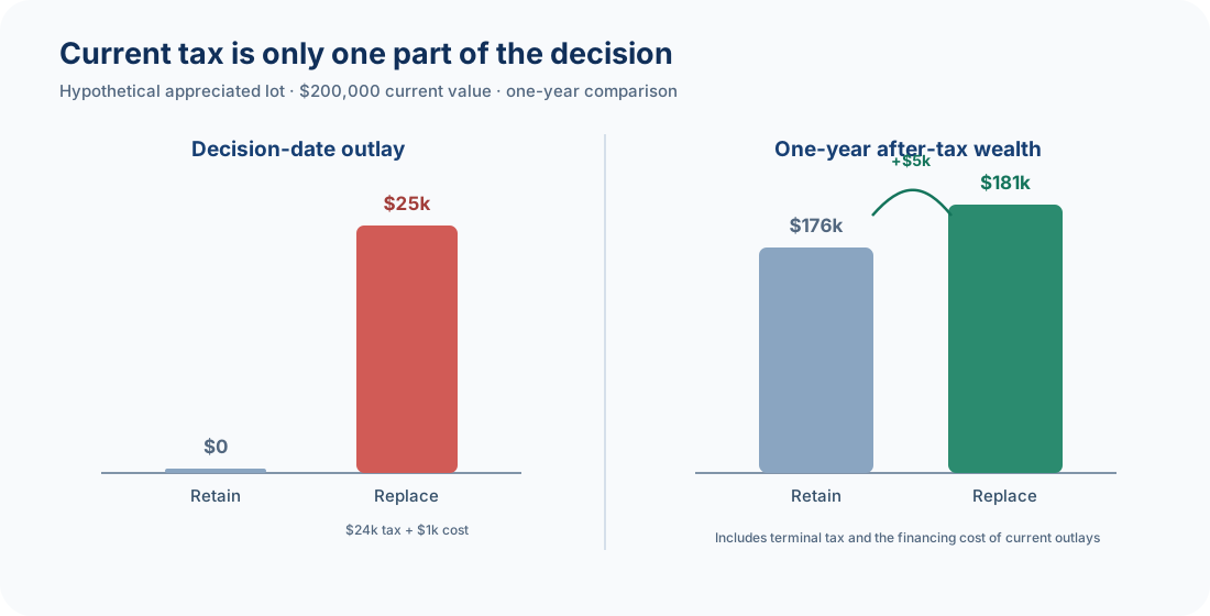
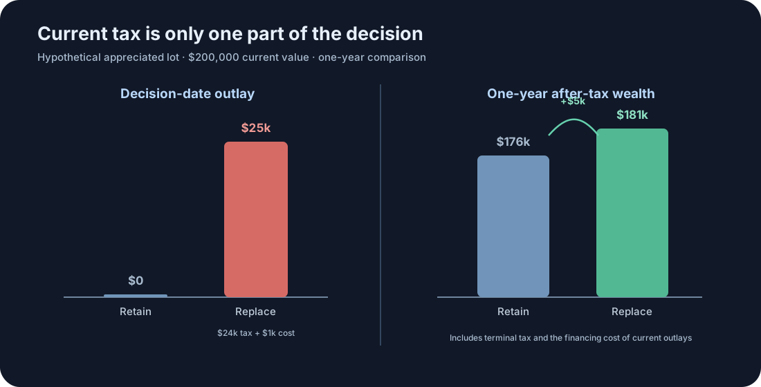
Assume a 30% policy rate, USD 1,000 of implementation cost, and a one-year replacement forecast of USD 210,000. The incumbent is forecast to remain at USD 200,000. Both paths are valued as if liquidated after one year, and current outlays carry a 4% financing cost.
Hypothetical one-year comparison
| Cash or value | Retain incumbent | Buy replacement |
|---|---|---|
| Current realized tax | USD 0 | USD 24,000 |
| Terminal pre-tax value | USD 200,000 | USD 210,000 |
| Terminal tax | USD 24,000 | USD 3,000 |
| Terminal value of current tax and cost | USD 0 | USD 26,000 |
| Terminal-equivalent after-tax wealth | USD 176,000 | USD 181,000 |
The replacement has the larger tax payment today, yet it finishes USD 5,000 ahead after tax. Retaining the incumbent does not eliminate the USD 24,000 tax on the existing gain; it postpones it to the comparison date. The replacement adds USD 10,000 of pre-tax value and incurs USD 3,000 of tax on that new gain. The USD 1,000 implementation cost becomes USD 1,040 at the endpoint, and paying the original tax one year earlier gives up another USD 960 of financing value. The result is USD 5,000 of terminal-equivalent value added.
If the replacement were forecast to reach only USD 202,000, retaining the lot would win under the same assumptions. Tax awareness therefore changes the hurdle for a trade. The forecast, risk change, cost, and deferral period determine its direction.
The arithmetic can be reproduced without the full optimization model:
rate = 0.30
current_value = 200_000
current_basis = 120_000
replacement_terminal = 210_000
cost = 1_000
financing = 1.04

retain = current_value - rate * (current_value - current_basis)
current_tax = rate * (current_value - current_basis)
replacement_tax = rate * (replacement_terminal - current_value)
replace = replacement_terminal - replacement_tax - (current_tax + cost) * financing

assert retain == 176_000
assert replace == 181_000
A loss harvest still needs an investable replacement
Now consider a USD 150,000 industrial holding with USD 190,000 of adjusted basis and beta of 1.20. Selling it realizes a USD 40,000 loss. The manager wants to retain the same cash, sector, and beta exposure using three industrial replacements that the approved policy places outside the original security's substantially-identical group.
A cash-, sector-, beta-, and POV-feasible transition
| Security | Trade notional | Beta | Beta trade | POV maximum |
|---|---|---|---|---|
| A | −USD 150,000 | 1.20 | −USD 180,000 | USD 150,000 |
| B | +USD 60,000 | 0.90 | +USD 54,000 | USD 60,000 |
| C | +USD 60,000 | 1.50 | +USD 90,000 | USD 75,000 |
| D | +USD 30,000 | 1.20 | +USD 36,000 | USD 40,000 |
| Total | USD 0 | — | USD 0 | Within every limit |
The trade notionals sum to zero. Every security is in the industrial sector, so sector exposure is preserved. The beta trades also sum to zero, and each purchase remains within its maximum participation of volume, or POV, amount.
Without the liquidity limit, buying USD 75,000 each of B and C would close cash, sector, and beta exposure. B can absorb only USD 60,000 in the selected execution window. Adding D restores feasibility. This is an important portfolio point: the tax loss may be attractive, but the implementation still has to produce a portfolio the mandate permits and the market can absorb.
Suppose the approved policy makes USD 25,000 of loss currently usable at a 30% rate. The USD 40,000 loss then produces USD 7,500 of current tax benefit and USD 15,000 of carryforward. The carryforward can have future value, but it is not current cash. Its value depends on future gains and the policy in force when it is used.
Wash state can cross several rebalances
Tax effects do not always settle on the sale date. Suppose an account sells 1,000 shares at USD 80 from a lot with basis of USD 100 per share. The USD 20,000 loss enters pending state because a qualifying replacement may still arrive inside the policy window.
Twelve days later, the account buys 600 shares at USD 78 in the same declared identity group. A proportional USD 12,000 of loss is transferred into the replacement basis. The replacement lot therefore has USD 58,800 of adjusted basis: USD 46,800 of purchase cost plus the transferred USD 12,000.
Hypothetical multi-period wash ledger
| Date | Event | Ledger consequence |
|---|---|---|
| Day 0 | Sell 1,000 at USD 80 | USD 20,000 loss pending; original quantity leaves the lot. |
| Day 12 | Buy 600 at USD 78 | USD 12,000 transferred; replacement basis becomes USD 58,800. |
| Expiry | No further replacement | Remaining USD 8,000 becomes recognized loss. |
| Later | Sell 600 at USD 105 | USD 63,000 proceeds less USD 58,800 basis produces USD 4,200 gain. |
The transferred USD 12,000 remains in adjusted basis. Without the basis adjustment, the later gain would have been USD 16,200. With the adjustment, it is USD 4,200. If the remaining USD 8,000 is fully usable at a 30% policy rate when the window expires, that expiry transition creates a USD 2,400 current benefit.
This sequence is why a multi-period system needs pending quantity, pending loss, replacement capacity, and future-lot basis. A one-day coefficient can help rank candidate sales, but the ledger must carry the unresolved event until later purchases or expiry determine its treatment.
For U.S. individual taxpayers, the IRS explains the relationship among sales, holding period, adjusted basis, and wash-sale basis adjustments in Publication 550. The numerical policy used here is deliberately simplified; an account's approved policy determines the treatment used by the optimizer.
Who pays the tax changes portfolio cash
Return to the appreciated-lot replacement and give the portfolio USD 1,000 of opening cash. Selling USD 200,000 and buying USD 200,000 is pre-tax cash-neutral. The trade also has USD 1,000 of implementation cost and USD 24,000 of realized tax.
The same tax liability under two payment modes
| Cash consequence | Tax paid externally | Tax paid by portfolio |
|---|---|---|
| Opening portfolio cash | USD 1,000 | USD 1,000 |
| Net security-trade cash | USD 0 | USD 0 |
| Implementation cost | −USD 1,000 | −USD 1,000 |
| Tax paid from portfolio | USD 0 | −USD 24,000 |
| Closing portfolio cash | USD 0 | −USD 24,000 |
| Investor's consolidated outlay | USD 25,000 | USD 25,000 |
External payment leaves the portfolio at its zero-cash floor while the investor pays USD 24,000 elsewhere. Portfolio payment breaks that floor. The account must raise another USD 24,000, receive an external contribution, or make a smaller replacement purchase.
The investor's consolidated outlay is USD 25,000 in both cases. Payment mode changes portfolio feasibility, not the economic existence of the tax. A report that shows only portfolio NAV can make external payment look cheaper, so the portfolio view and consolidated after-tax view need to be shown together.
What the portfolio manager should receive
A useful decision record separates quantities that answer different questions.
Decision and performance views
| Measure | Question it answers |
|---|---|
| Market P&L | What did the positions earn while they were held? |
| Realized character | Which embedded gains and losses changed tax status? |
| Implementation cost | What did the transition cost to execute? |
| Current tax cash | What is payable or currently usable under the selected policy? |
| Deferred liquidation tax | What tax remains attached to the ending lots under the declared endpoint? |
| After-tax value added | Did the tax-aware policy improve consolidated wealth versus a named reference? |
| Constraint residuals | Did cash, sector, beta, equality, and POV controls actually close? |
The reference policy matters. A comparison might use a tax-agnostic target rebalance, a simple highest-basis-first rule, or the account's existing process. It should be named before the evaluation begins. Otherwise, “tax alpha” can become whatever difference happens to favor the selected method.
From hypothetical fixtures to empirical evidence
These examples establish accounting signs and portfolio mechanics. An empirical study would go further. It would freeze the opening lots, policy, market data, forecasts, constraints, and reference decision at each historical cutoff; run the exact and faster methods from the same eligible state; apply their actual or simulated fills to separate ledgers; and compare later market P&L, implementation cost, current tax, deferred tax, tracking risk, and liquidation wealth.
Results would be reported across accounts, dates, market regimes, gain and loss states, liquidity levels, and holding-period boundaries. The hypothetical fixtures remain useful inside that study because every empirical transition still has to conserve quantity and basis and close its mandate residuals.
The companion StrategyNet white paper in the White Papers section gives the complete multi-period formulation, state definitions, deterministic ledger, exact-reference comparison, and test contract behind these examples.
Common questions
Is the highest-basis lot always the best lot to sell?
No. It often produces less current gain, but it also leaves lower-basis lots and their deferred tax in the account. Character, holding-period boundaries, loss capacity, wash exposure, and the desired terminal portfolio can change the ranking.
Does cash neutrality fund tax and transaction cost?
Pre-tax cash neutrality means gross purchases equal gross sales. Tax and implementation cost still need funding. The payment-mode example shows why the cash ledger is separate from the trade-notional equality.
Is every harvested loss worth its rate times the loss?
Only the portion currently usable under the approved policy creates current benefit. The remainder may become carryforward or pending state. A qualifying replacement may transfer some loss into basis rather than producing current tax cash.
Why optimize more than one period if only today's trade is executed?
Later periods let today's decision see holding-period changes, future cash needs, loss use, liquidity, and unresolved wash state. The next decision is then solved again from observed holdings and the reconciled ledger.
Further reading
This walkthrough is for research and educational purposes. It illustrates how strategynet.ai organizes signal evidence into factors and scenarios. It provides no recommendation, investment advice, or instruction to trade any security.
Back to Insights