Jörmungandr: Plugin-Based Distributed Reinforcement Learning

Jörmungandr is a reinforcement-learning framework with replaceable training algorithms and a shared lifecycle for data collection, evaluation, checkpointing, and inference. Keeping those surrounding processes consistent helps researchers attribute measured differences to the algorithms being compared.

This article explains the experiment lifecycle, the data requirements of its algorithm families, and the available comparisons and reproducible materials. The release registers C51, QR-DQN, DQN, discrete CQL, maximum-entropy Soft-Q, behavior cloning, MARWIL, PPO, IMPALA, APPO/IMPACT, categorical SAC, and a compact vector-observation DreamerV3 profile. It is released under Apache-2.0. The Python distribution is jormungandr-rl; its import name is jormungandr.

The stable experiment boundary

An actor observes \(o_t\), chooses action \(a_t\) under policy version \(v\), receives reward \(r_t\), and observes \(o_{t+1}\). Jörmungandr records

\[\tau_t = (o_t,a_t,r_t,o_{t+1},d_t; \text{actor},\text{episode},t,\text{split},v, \log \mu_v(a_t\mid o_t),V_v(o_t)),\]

where \(d_t\) records termination and the last two fields retain behavior-policy information when an algorithm requires it. Legal-action masks and external state references can travel with the same record.

Training and validation samples may be interleaved in one request. Routing is a property of each transition rather than its connection or arrival time. Training data update the training-only observation normalizer and enter replay; validation data enter a separate bounded store and cannot change weights, priorities, or normalization. The experience protocol defines the complete wire contract.

The learner plugin exchanges NumPy arrays and plain mappings with the runtime. Its action result can include the action index, log probability, value, and algorithm-specific diagnostics. Its update result returns a normalized loss, one replay priority per sampled item, and named metrics. This boundary allows a Torch implementation today and a future native selector or replay kernel without changing actor messages.

Algorithms use different valid data units

The plugin catalogue does not make every algorithm directly comparable. Online value learners—DQN, C51, QR-DQN, Soft-Q, and categorical SAC—can consume the same one-step transition stream. PPO needs fresh behavior-policy trajectories. IMPALA and APPO correct bounded actor lag using V-trace-style importance ratios. BC, CQL, and MARWIL require a declared offline behavior or demonstration dataset. DreamerV3 learns from sequences and consumes an additional model-training budget.

Jörmungandr therefore supports two replay modes. Transition learners draw one-step samples from ordinary prioritized replay or a pluggable selector. Trajectory learners assemble contiguous fragments by actor, episode, timestep, and policy version. A stale transition can be recorded for audit while being excluded from an on-policy update.

Each checkpoint retains the model configuration, algorithm name and semantic plugin version, plugin-owned state, optimizer state, training normalizer, feature order, policy version, and learner counters. Restore rejects a silent algorithm mismatch. Replay and validation contents are intentionally not part of the model checkpoint; resuming the same model is distinct from reproducing the exact interrupted data stream.

Noise and return risk

Noise has several meanings in reinforcement learning. Reward outliers alter a TD target; observation error changes the estimated state; stochastic dynamics widen the return distribution; an offline dataset changes action support; and distributed actors create policy lag. No algorithm name resolves all five.

The value profiles use Huber losses, gradient clipping, Double-DQN targets, and optional reward clipping or observation augmentation where appropriate. Categorical C51 retains a discrete return distribution. QR-DQN learns quantile locations and can deploy the mean, a fixed lower quantile, or lower-tail CVaR score. Twin critics in categorical SAC address optimistic value bias, while CQL addresses unsupported actions in offline data.

Maximum-entropy RL supplies a more specific robustness hypothesis. Eysenbach and Levine show that an entropy-regularized objective lower-bounds robust objectives for characterized reward and transition perturbation sets. That result does not imply robustness to every sensor error or market regime. The temperature, disturbance family, and evaluation cohort still belong in the experiment.

QUBO allocates an expanded frontier

Jörmungandr can use quadratic unconstrained binary optimization (QUBO) to choose which replay fragments or search candidates receive a limited budget. For normalized utility \(u_i\), pairwise similarity \(s_{ij}\), and target count \(k\), the implemented energy is

\[E(x)= -\lambda_u\sum_i u_i x_i +\lambda_s\sum_{i<j}s_{ij}x_ix_j +\lambda_k\left(\sum_i x_i-k\right)^2, \qquad x_i\in\{0,1\}.\]

The linear term rewards useful candidates; the pair term charges for retaining redundant paths; the final term enforces the budget. The built-in solver is a deterministic classical greedy construction followed by one-for-one local exchanges. It exports the Q matrix and decision audit so another classical, annealing, or native backend can replace only the solve step.

The search statement is precise. At depth \(t\), the retained beam \(\mathcal B_{t-1}\) is expanded into one complete candidate frontier \(\mathcal C_t\). One QUBO over \(\mathcal C_t\) produces the binary vector \(x_t\), and candidates with \(x_{t,i}=1\) become \(\mathcal B_t\). QUBO is not solved independently inside each branch.

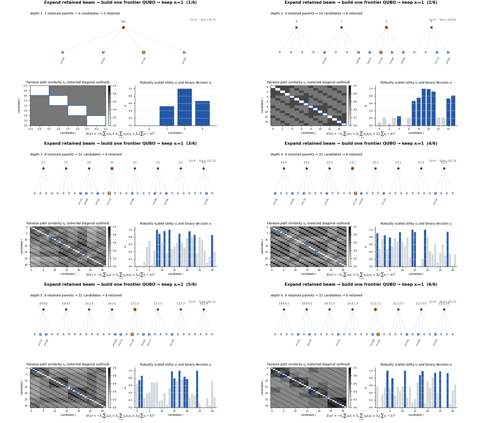
The controlled benchmark constructs 500 paired four-way trees of depth six. Search receives a cheap value proxy whose error is correlated within the first branch, while the benchmark retains all 4,096 terminal values for scoring. At beam width eight, utility-only search recovered the exact optimum in 72.2% of trials with mean regret 0.1435. QUBO recovered 73.2% with mean regret 0.1305. The paired mean-regret improvement was 0.0130 with a normal 95% interval from 0.0022 to 0.0239.

QUBO selection averaged 2.87 ms at that width versus 0.09 ms for utility-only selection. Matching aggregate quality against a utility beam of width ten saved 32 generated candidates and two terminal evaluations. Ignoring candidate generation cost, each avoided terminal evaluation must cost about 1.38 ms for the selector overhead to break even. This is evidence for the integration on the declared synthetic noise model, not general QUBO or quantum advantage.

Comparing compatible online agents

The first learning comparison holds the data contract fixed. DQN, C51, QR-DQN, maximum-entropy Soft-Q, and categorical SAC each receive five independently initialized runs, 64 training episodes of 32 steps, and the same training-path schedule. After a 128-transition warm-up, each run makes one update per new transition, for 1,921 updates. Every checkpoint is evaluated without learning on the same 16 held-out paths.

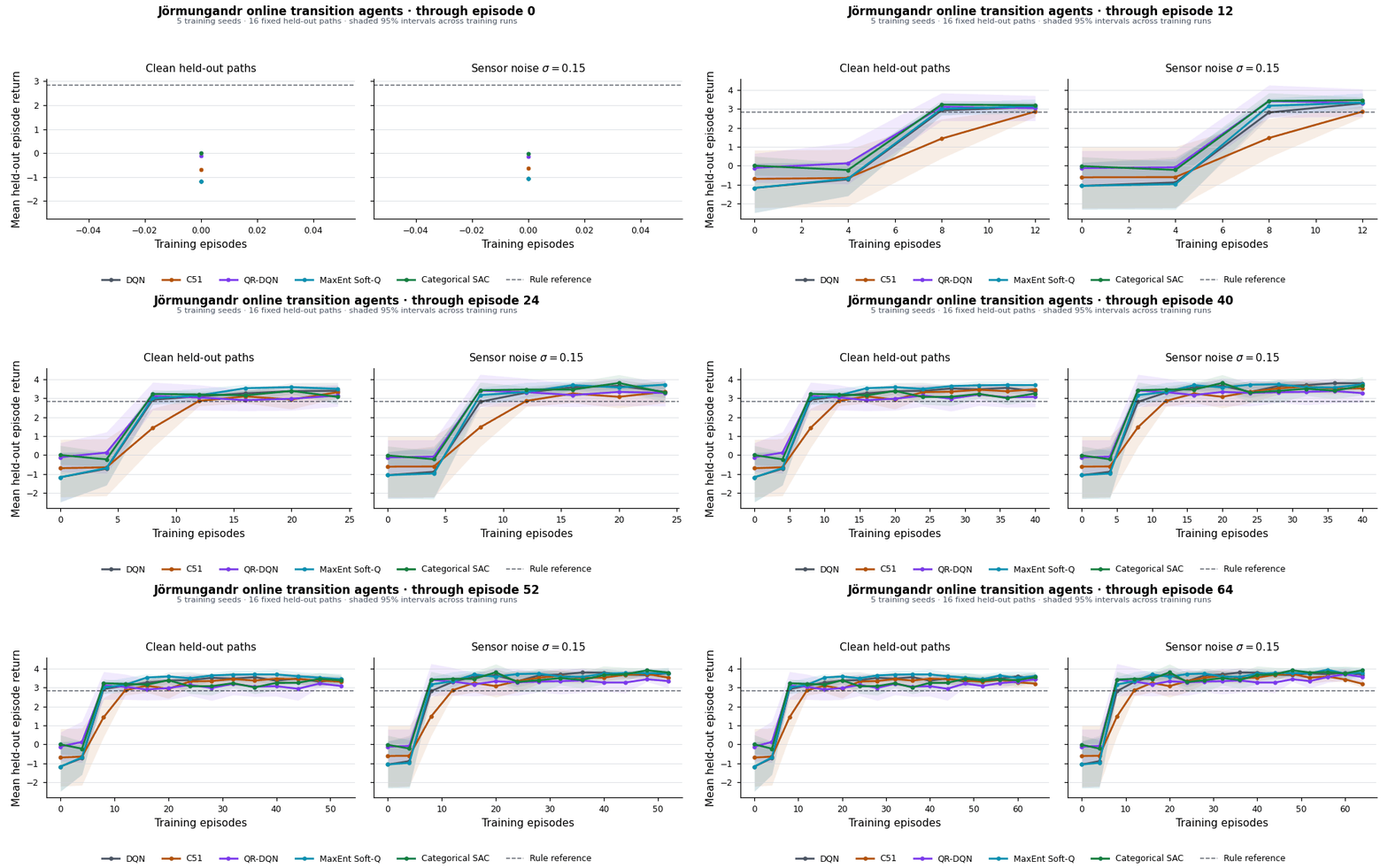
The rule reference returns 2.8367 on the held-out paths. Final clean-return point estimates are 3.4413 for DQN, 3.2101 for C51, 3.4382 for QR-DQN, 3.6087 for Soft-Q, and 3.5508 for SAC. Soft-Q has the largest clean point estimate and SAC the largest sensor-noise point estimate, but several intervals overlap. Noise also improves some point estimates in this threshold-like environment. The study demonstrates the comparison protocol and behavioral differences; it does not establish a general winner or a noise-robustness guarantee.

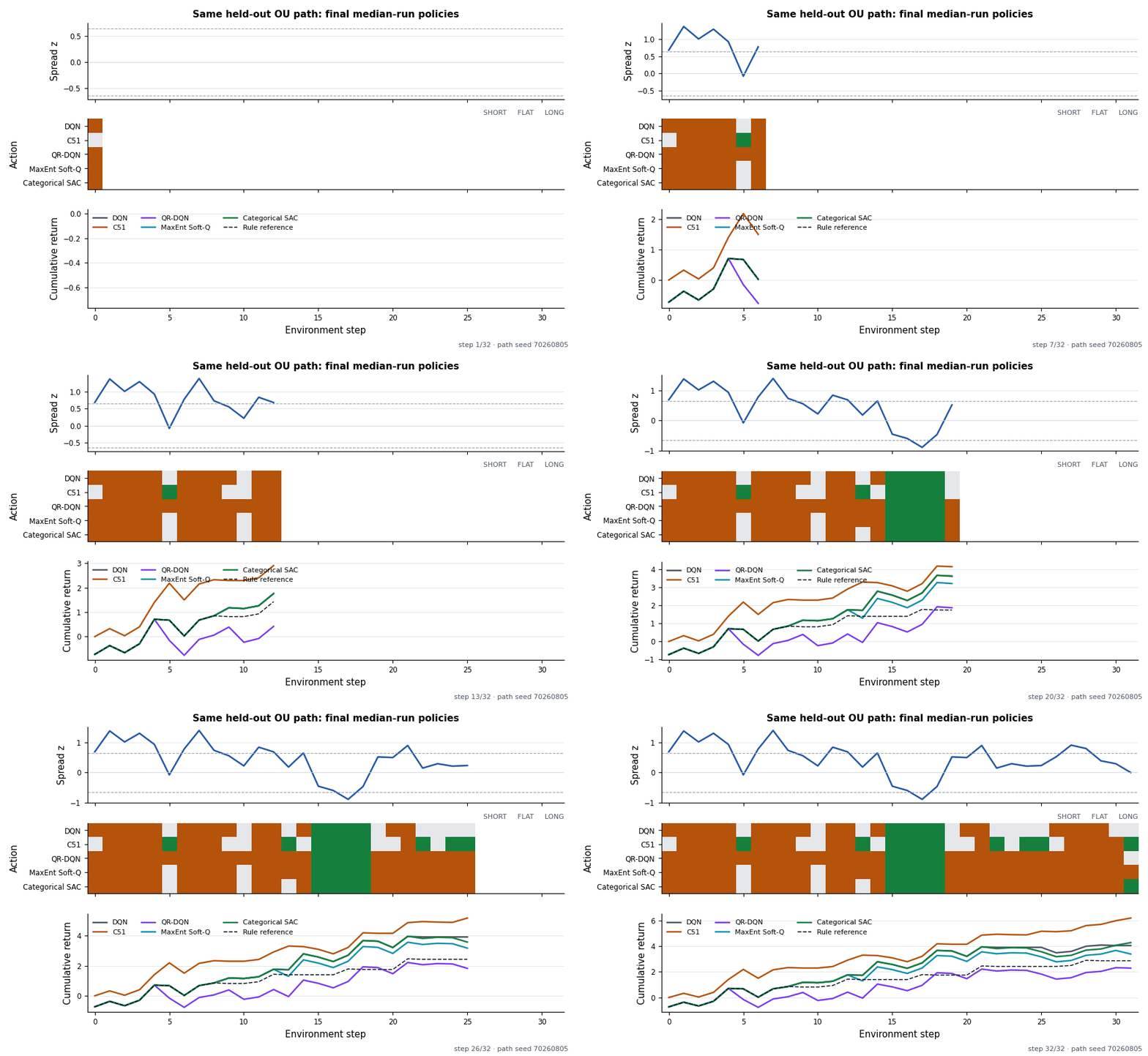
The synthetic OU process is independent of the chosen action, so every policy in the playback receives the same exogenous spread path. Actions still affect position, turnover cost, reward, and the next observation. A single playback is useful for diagnosis but cannot replace the repeated held-out evaluation.

Volt policies and a future native boundary

Volt can use a frozen Deep Sets or graph embedding through the fixed-vector service today. End-to-end Torch Deep Sets and GNN policies can train through Jörmungandr's in-process masked-policy boundary, preserving gradients through the encoder. Graph-native HTTP batching, dynamic action descriptors, and a checkpointed graph artifact store remain future work.

Python remains the orchestration and research layer. Policy modules, automatic differentiation, and optimizers remain in Torch. Replay indexing, trajectory assembly, QUBO construction and local search, graph collation, GAE, and V-trace are plausible Rust/PyO3 candidates after profiling. Keeping the plugin boundary in arrays and mappings allows those kernels to move without creating a second policy or checkpoint ecosystem.

The release has 48 functional tests, including finite updates and state round trips for every built-in plugin, validation isolation, legal masks, trajectory assembly, QUBO cardinality and frontier accounting, checkpoint restore, TorchScript manifests, and the seeded comparison harness. These lifecycle and synthetic studies do not reproduce Atari, continuous-control, offline-RL, Minecraft, or Volt trading benchmarks.

Paper and reproducible materials

Read Jörmungandr: A Plugin Runtime for Distributed Reinforcement Learning, the 16-page paper containing the plugin contracts, mathematical QUBO formulation, empirical branch study, convergence comparison, Volt boundary, and staged Rust path. The source, benchmark JSON, and plotting scripts are published with the implementation.

References

• Marc G. Bellemare, Will Dabney, and Rémi Munos, A Distributional Perspective on Reinforcement Learning, Proceedings of Machine Learning Research 70, 2017.
• Will Dabney et al., Distributional Reinforcement Learning with Quantile Regression, 2018.
• Benjamin Eysenbach and Sergey Levine, Maximum Entropy RL (Provably) Solves Some Robust RL Problems, International Conference on Learning Representations, 2022.
• Tuomas Haarnoja et al., Soft Actor-Critic, International Conference on Machine Learning, 2018.
• Lasse Espeholt et al., IMPALA: Scalable Distributed Deep-RL with Importance Weighted Actor-Learner Architectures, 2018.

Continue with Volt, the open-source options portfolio library, Hypercube, the open-source live analytics engine, or browse the Jörmungandr source.