
Data Mining in Nonstationary Markets
Repeated strategy testing raises the chance of selecting a result produced by sampling noise. Changing market conditions add uncertainty about whether a historical relationship will persist. Together, these problems affect how much confidence researchers can place in a successful backtest.
This article explains how specification search and nonstationarity influence research conclusions. It uses a seeded selection-bias simulation, examines replication evidence, and sets out a protocol for recording trials, separating selection from evaluation, and testing stability through time.
Where data mining enters a backtest
Test 100 independent, useless strategy variants at a 5% significance level. The probability that at least one passes by chance is
\[1-(1-0.05)^{100}=99.4\%.\]
Reporting the winner's \(p\)-value as if it came from one planned test discards the search that produced it. Financial research creates this problem whenever the same market history guides the choice of signal, lag, universe, horizon, normalization, neutralization, cost model, and sample period.
Nonstationarity adds a second problem. The relationship that generated returns during the backtest can weaken, reverse, or disappear as participants, policy, market structure, data definitions, and implementation costs change. A clean historical test can estimate yesterday's process accurately and still provide a poor forecast of tomorrow's process.
Exploration generates hypotheses and is essential to research. The evidential error occurs when observations used to choose a specification are presented again as fresh evidence for that specification. The search includes every decision whose choice depended on the results, including decisions made outside the code.
A single reported backtest may contain a large hidden search
| Research choice | Examples | Trial record required |
|---|---|---|
| Signal definition | raw field, transform, direction, interaction, missing-value rule | every evaluated definition and version |
| Target | return horizon, close-to-close or open-to-close, excess or raw return | every label and execution lag |
| Universe | region, liquidity cutoff, sector exclusions, surviving securities | point-in-time membership rule |
| Construction | rank or z-score, neutralization, weighting, position limits | complete portfolio recipe |
| Evaluation | start date, end date, benchmark, metric, cost assumption | planned rule and all observed outcomes |
Trying 20 horizons in one program and trying them across 20 successive research meetings create the same selection problem. Correlation changes the effective number of trials and the appropriate adjustment. A registry should retain the full family and the order in which results became visible.
Why nonstationarity makes selection more dangerous
Consider a predictive relationship
\[R_{t+1}=\alpha_t+\beta_t x_t+\varepsilon_{t+1}.\]
A full-sample regression compresses the path of \(\beta_t\) into one estimate. That average can conceal a strong relationship followed by a weak one, a sign change, or a short episode that dominates the result. The causes can enter at several levels:
- Measurement: a vendor revises a field, reporting lags change, or universe coverage expands.
- Population: the mix of securities, participants, and liquidity changes.
- Payoff mapping: the same observation leads to different subsequent returns under a new policy or market regime.
- Implementation: crowding, capacity, borrow availability, fees, and execution technology alter realized returns.
- Response to discovery: capital trades against a published or deployed relationship and reduces its payoff.
A decaying backtest therefore admits several explanations: initial selection bias, structural change, implementation crowding, data revision, or cost drift. The retained research record is what allows those explanations to be tested separately.
A holdout can become part of the search
Temporal train and test periods help only while the later period remains untouched. A researcher who checks the test result, changes the feature set, and checks again has started fitting to that test period. Team memory can contaminate a nominally new experiment even when the code uses a clean split.
Random cross-validation also changes the question for time-ordered data. Shuffling observations lets future regimes inform earlier fits and can place overlapping return labels on both sides of a split. Forward splits, explicit gaps for overlapping labels, and point-in-time feature construction preserve the information sequence faced by the historical decision.
An untouched period remains a finite sample. A short test may miss a weak signal, reward a lucky one, or contain only one regime. External evidence across markets and a later shadow or live period provide additional tests, each with its own differences in population and implementation.
What specification search does under a pure null
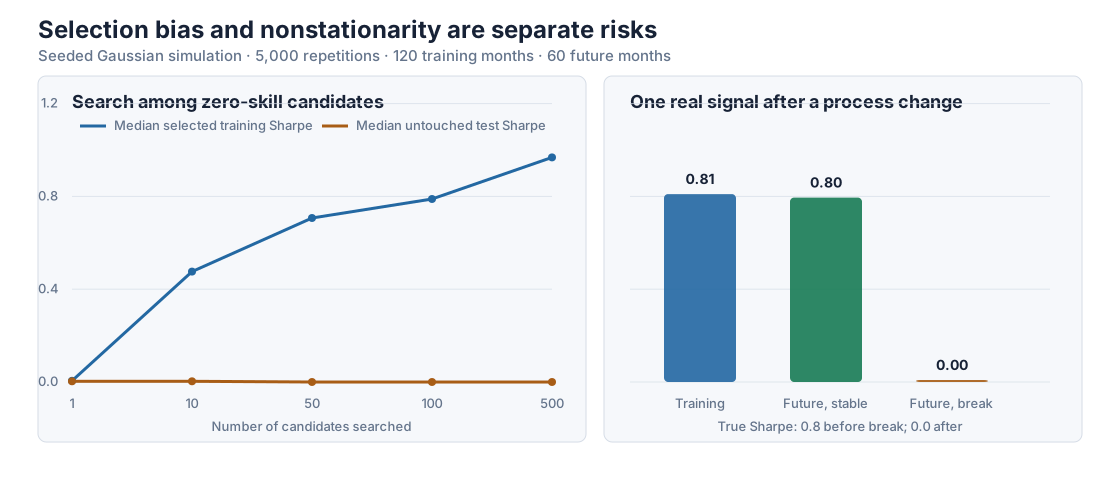
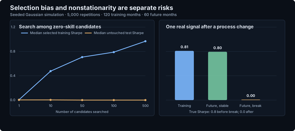
The following simulation gives every candidate a true expected return of zero. For each of 5,000 repetitions, it estimates annualized Sharpe ratios over 120 monthly observations, selects the highest, and evaluates the selected candidate on 60 new monthly observations.
Seeded Gaussian simulation under zero true Sharpe
| Candidates searched | Median selected training Sharpe | 90th percentile training Sharpe | Median untouched test Sharpe | Test Sharpe below zero |
|---|---|---|---|---|
| 1 | 0.005 | 0.416 | 0.003 | 49.8% |
| 10 | 0.476 | 0.740 | 0.003 | 49.6% |
| 50 | 0.707 | 0.931 | −0.010 | 50.9% |
| 100 | 0.789 | 0.999 | −0.002 | 50.3% |
| 500 | 0.968 | 1.151 | −0.012 | 51.0% |
Searching 500 zero-skill candidates produces a median winning in-sample Sharpe of 0.968. The same selected candidates have a median Sharpe of −0.012 on new data. Selection created the apparent performance.
The right panel introduces a different failure. A signal has a true annual Sharpe of 0.8 during training. When the process remains stable, the median future estimate is 0.795. After a structural break sets the true Sharpe to zero, the median future estimate is 0.003. The training procedure was sound; the payoff process changed.
The core calculation can be reproduced by drawing each null Sharpe from its finite-sample \(t\) distribution:
from math import sqrt
from random import Random
from statistics import median

rng = Random(20260723)
repetitions = 5_000
train_months, test_months = 120, 60

def null_sharpe(months):
    degrees = months - 1
    t_value = rng.gauss(0, 1) / sqrt(
        rng.gammavariate(degrees / 2, 2) / degrees
    )
    return t_value * sqrt(12 / months)

selected_train, selected_test = [], []
for _ in range(repetitions):
    selected_train.append(max(null_sharpe(train_months) for _ in range(500)))
    selected_test.append(null_sharpe(test_months))

print(round(median(selected_train), 3))  # 0.968
print(round(median(selected_test), 3))   # about 0
The simulation assumes independent Gaussian candidates and returns. Real strategies share inputs, exposures, and observations; their dependence changes the distribution of the maximum. The example isolates the selection mechanism; a universal Sharpe haircut would require a stated joint distribution and search process.
Research controls that address distinct failures
No single statistic repairs an unrestricted research process. Each control below addresses a specific way that information can leak into the reported result.
Controls for a signal research programme
| Control | Failure addressed | Evidence retained |
|---|---|---|
| Hypothesis and family registration | result-driven direction, horizon, universe, or benchmark changes | economic rationale, search family, planned metric, rejection rule |
| Point-in-time data contract | look-ahead and survivorship bias | observation time, availability time, universe membership, revision version |
| Nested forward validation | fitting hyperparameters to the reported test | inner selection windows, outer evaluation windows, overlap gaps |
| Complete trial ledger | hidden researcher degrees of freedom | every candidate, parameter set, run time, outcome, and parent experiment |
| Multiplicity-aware inference | choosing the best result from a family | family definition, dependence assumptions, adjusted result |
| Stability map | dependence on one episode or fragile parameter value | rolling estimates, subperiods, nearby parameters, influence diagnostics |
| Shadow and live monitoring | process change after research | frozen deployment version, expected range, decay trigger, review decision |
Register the question before measuring the winner
The record should specify the information available at the decision time, the forecast horizon, expected direction, eligible universe, benchmark, primary metric, and rejection gate. Exploratory variants remain visible as members of one search family. A later economic insight can justify a new specification, with a new version and a later evaluation period.
Run selection inside each historical training window
An honest walk-forward test repeats the entire research decision. At each outer rebalance, feature selection, hyperparameter tuning, normalization, model fitting, and portfolio calibration use earlier observations. The next outer period supplies one evaluation. Return windows that overlap the boundary require a gap or explicit dependence treatment.
Match the statistical method to the search
False-discovery-rate procedures estimate the share of false discoveries among a declared family under their dependence assumptions. White's Reality Check and Hansen's Superior Predictive Ability test compare a searched set of forecasting models with a benchmark. Probability of Backtest Overfitting examines how often the selected in-sample winner underperforms across combinatorial out-of-sample splits. A complete walk-forward run evaluates the actual model-selection pipeline.
These methods ask different questions. Their inputs must include the models that lost the search, and their assumptions should be reported with the result.
Test stability before averaging it away
Report rolling efficacy, sign by subperiod, universe and sector contributions, performance near the chosen parameter values, turnover, and cost sensitivity. A factor whose full-period mean depends on one short interval or a few securities needs that concentration stated explicitly.
Monitoring rules belong in the research specification. A rule may trigger review when rolling efficacy leaves its expected range, coverage changes, implementation costs exceed the research allowance, or factor exposures drift. Automatic reversal after a bad period creates another searched strategy.
What empirical replication studies show
Published replication studies report materially different failure rates.
McLean and Pontiff (2016) studied 97 return predictors and reported average portfolio returns 26% lower out of sample and 58% lower after publication. Their design attributes the out-of-sample decline partly to statistical bias and the additional post-publication decline partly to investor learning.
Hou, Xue, and Zhang (2020) applied consistent construction rules to 452 anomalies. They reported that 65% failed a conventional single-test hurdle and 82% failed their multiple-test hurdle, with microcap treatment and weighting choices materially affecting the results.
Jensen, Kelly, and Pedersen (2023) used a Bayesian framework and a global data set of 153 factors across 93 countries. They concluded that a majority of factors replicated and that the factor zoo could be organized into a smaller set of themes.
Goyal, Welch, and Zafirov (2024) revisited 46 equity-premium predictors using common specifications and real-time out-of-sample tests. Only a minority retained useful performance, and the authors documented pronounced variation through time.
Different hypotheses, construction rules, samples, and inferential frameworks produce different answers. A research system should preserve those choices alongside the result so that “replication” has an exact operational meaning.
The research record StrategyNet should require
A promoted factor should retain:
- the economic hypothesis and expected direction;
- the complete versioned calculation and point-in-time data contract;
- the parent search family and every evaluated sibling;
- the inner selection and outer evaluation dates;
- the planned benchmark, costs, metrics, and rejection gates;
- multiplicity, dependence, stability, and influence diagnostics;
- the frozen version used in shadow or live evaluation; and
- every later retain, revise, suspend, or retire decision.
This record makes a current score traceable to the exact evidence that admitted its factor version. When efficacy decays, the same lineage shows whether the change came from inputs, population, payoff mapping, implementation, or the original search.
Sources
- Halbert White, “A Reality Check for Data Snooping”, Econometrica 68(5), 2000.
- Peter R. Hansen, “A Test for Superior Predictive Ability”, Journal of Business & Economic Statistics 23(4), 2005.
- Campbell R. Harvey, Yan Liu, and Heqing Zhu, “… and the Cross-Section of Expected Returns”, Review of Financial Studies 29(1), 2016.
- David H. Bailey, Jonathan M. Borwein, Marcos López de Prado, and Qiji Jim Zhu, “The Probability of Backtest Overfitting”, Journal of Computational Finance 20(4), 2017.
- Rob Arnott, Campbell R. Harvey, and Harry Markowitz, “A Backtesting Protocol in the Era of Machine Learning”, Journal of Financial Data Science 1(1), 2019.
Next reading
This walkthrough is for research and educational purposes. It illustrates how strategynet.ai organizes signal evidence into factors and scenarios. It provides no recommendation, investment advice, or instruction to trade any security.
Back to Insights