
When Is an Information Coefficient Reliable?
The reliability of an information coefficient depends on the uncertainty around its estimate and the research process that produced it. Assessing that uncertainty helps researchers judge how much evidence a measured relationship provides for using a signal.
This article examines two estimates: the correlation across securities on one date and the mean of those correlations through time. It explains how sample size, overlapping returns, serial dependence, and repeated testing affect the assessment, then works through a numerical example and a dependence-aware confidence interval.
The quantity whose reliability is being assessed
For the point-in-time eligible universe \(U_t\), define the date-level rank IC as
\[\rho_t = \operatorname{corr}_{i\in U_t} \left( \operatorname{rank}(f_{i,t}), \operatorname{rank}(R_{i,t\rightarrow t+h}^{(b)}) \right),\]
where \(f_{i,t}\) is the signal available at observation time \(t\) and \(R_{i,t\rightarrow t+h}^{(b)}\) is the subsequent return over horizon \(h\) in base currency \(b\). The universe, signal direction, horizon, lag, treatment of ties and missing pairs, and minimum valid security count must be fixed before the result is examined.
The population quantity usually sought in a historical IC study is the mean date-level association
\[\mu_{IC}=\mathbb{E}[\rho_t].\]
Given \(T\) completed observation dates, its sample estimate is
\[\widehat{\mu}_{IC}=\overline{\rho} =\frac{1}{T}\sum_{t=1}^{T}\rho_t.\]
Reliability refers to the uncertainty around this estimate under the research design. The estimate supplies no probability for success on the next date and contains no portfolio return; both require further analysis.
Uncertainty within one cross-section
Each \(\rho_t\) is estimated from \(N_t\) valid signal-return pairs. For Pearson correlation, a conventional large-sample interval uses Fisher's transformation
\[z_t=\operatorname{arctanh}(\rho_t), \qquad \operatorname{SE}(z_t)\approx\frac{1}{\sqrt{N_t-3}},\]
then transforms the interval endpoints back with \(\tanh(\cdot)\). This approximation relies on conditions that are rarely exact in security returns, including independent pairs and a suitable joint distribution.
Rank IC has a different sampling distribution. An unrestricted asymptotic \(p\)-value can be inaccurate in a small cross-section, especially with ties. A permutation test or bootstrap is often more informative, provided its resampling scheme preserves the structure that should remain under the null. For example, an unrestricted shuffle assumes that security labels are exchangeable; strong sector or issuer dependence can make that assumption unreasonable.
The valid security count should accompany every date-level IC. A correlation from 18 pairs and one from 1,800 pairs may have the same value while carrying very different sampling uncertainty. Common market and sector exposures also mean that the effective cross-sectional information can be smaller than the security count.
Uncertainty in mean IC through time
If the \(T\) date-level IC observations were independent and identically distributed, the ordinary standard error would be
\[\operatorname{SE}_{\mathrm{ordinary}} =\frac{s_{IC}}{\sqrt{T}},\]
where \(s_{IC}\) is their sample standard deviation. Daily and weekly IC series often violate the independence assumption. Persistent signals, repeated universe membership, common market conditions and overlapping forward-return windows can cause nearby observations to move together.
A heteroskedasticity and autocorrelation consistent estimate allows recent autocovariances to contribute to the standard error. With Bartlett weights and bandwidth \(L\), define
\[\widehat{\gamma}_{\ell} = \frac{1}{T} \sum_{t=\ell+1}^{T} (\rho_t-\overline{\rho})(\rho_{t-\ell}-\overline{\rho}),\]
and
\[\operatorname{SE}_{HAC} = \sqrt{ \frac{1}{T} \left[ \widehat{\gamma}_0 +2\sum_{\ell=1}^{L} \left(1-\frac{\ell}{L+1}\right) \widehat{\gamma}_{\ell} \right] }.\]
An approximate two-sided confidence interval is
\[\overline{\rho} \ \pm\ z_{1-\alpha/2}\operatorname{SE}_{HAC}.\]
The bandwidth is part of the method and should be recorded. A five-day return calculated every day creates at least four days of mechanical label overlap, although signal persistence and market regimes can extend dependence beyond that span. In a short sample or a series with strong dependence, a moving-block or stationary bootstrap can provide a useful comparison with the asymptotic interval.
A numerical example with serial dependence
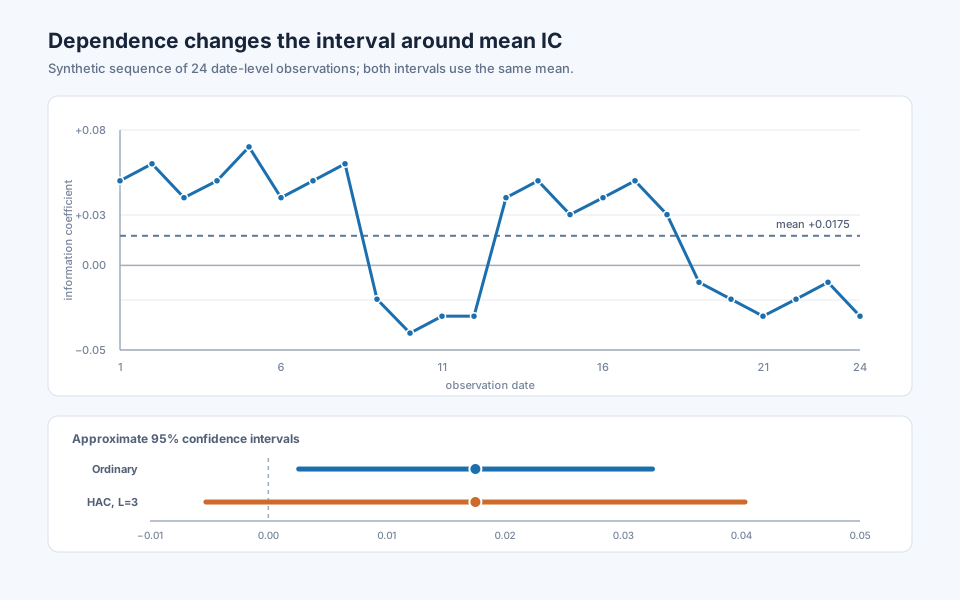
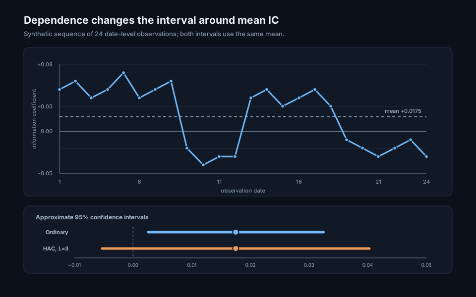
Consider 24 synthetic date-level IC observations. Positive and negative values occur in clusters, as can happen when one market condition lasts for several observations.
Synthetic date-level information coefficients
| Dates | IC observations |
|---|---|
| 1–8 | +0.05, +0.06, +0.04, +0.05, +0.07, +0.04, +0.05, +0.06 |
| 9–12 | −0.02, −0.04, −0.03, −0.03 |
| 13–18 | +0.04, +0.05, +0.03, +0.04, +0.05, +0.03 |
| 19–24 | −0.01, −0.02, −0.03, −0.02, −0.01, −0.03 |
The mean IC is \(0.0175\). Treating the dates as independent gives a standard error of \(0.0076\) and an approximate 95% interval from \(0.0026\) to \(0.0324\). A Bartlett HAC calculation with three lags gives a standard error of \(0.0116\) and an interval from \(-0.0053\) to \(0.0403\).
The ordinary interval excludes zero; the dependence-aware interval includes zero. The estimated mean remains \(0.0175\) in both calculations. Their standard errors differ because they assign different amounts of independent information to the 24 dates. This is an illustrative sequence, and 24 observations would be too short to settle an empirical claim.
Python calculation
from math import sqrt
from statistics import mean, stdev

ic = [
    0.05, 0.06, 0.04, 0.05, 0.07, 0.04, 0.05, 0.06,
    -0.02, -0.04, -0.03, -0.03,
    0.04, 0.05, 0.03, 0.04, 0.05, 0.03,
    -0.01, -0.02, -0.03, -0.02, -0.01, -0.03,
]

sample_size = len(ic)
mean_ic = mean(ic)
ordinary_se = stdev(ic) / sqrt(sample_size)

centered = [value - mean_ic for value in ic]
gamma_0 = sum(value * value for value in centered) / sample_size
bandwidth = 3
long_run_variance = gamma_0

for lag in range(1, bandwidth + 1):
    gamma = sum(
        centered[index] * centered[index - lag]
        for index in range(lag, sample_size)
    ) / sample_size
    bartlett_weight = 1 - lag / (bandwidth + 1)
    long_run_variance += 2 * bartlett_weight * gamma

hac_se = sqrt(long_run_variance / sample_size)
z_95 = 1.96

print("mean", round(mean_ic, 4))
print("ordinary", round(ordinary_se, 4),
      tuple(round(mean_ic + sign * z_95 * ordinary_se, 4)
            for sign in (-1, 1)))
print("HAC", round(hac_se, 4),
      tuple(round(mean_ic + sign * z_95 * hac_se, 4)
            for sign in (-1, 1)))

# mean 0.0175
# ordinary 0.0076 (0.0026, 0.0324)
# HAC 0.0116 (-0.0053, 0.0403)
Interpreting positive, zero and negative estimates
A positive mean with an interval comfortably above zero supports the registered positive signal direction under the stated sampling model. An interval that includes zero means that the data and method do not rule out a null average at the selected confidence level. It can accompany a positive point estimate when the sample is short, volatile or dependent.
A negative estimate can indicate that the signal orientation was wrong, that the relationship changed during the test, or that sampling variation dominated a weak forecast. Its interval and period-by-period history help distinguish a persistent inverse relationship from an isolated adverse episode. Reversing the signal after reading the result creates a new hypothesis that needs a later, untouched evaluation period.
Confidence intervals also have sampling variation. Passing or failing a single zero threshold should not replace examination of stability across time, coverage, economic rationale and implementation.
Overlapping horizons and effective sample size
Suppose a signal is observed daily and tested against the next five trading days' return. The label for Monday shares four daily returns with the label for Tuesday. Adjacent IC observations can therefore be correlated even if the signal itself changes each day. Counting both dates as fully independent makes the ordinary standard error too optimistic when those autocovariances are positive.
For a stationary series, the diagnostic approximation
\[T_{\mathrm{eff}} \approx \frac{T} {1+2\sum_{\ell=1}^{L}\operatorname{corr}(\rho_t,\rho_{t-\ell})}\]
shows how positive serial correlation reduces the effective number of dates. This value can be unstable when the sample is short or the lag correlations are noisy, so it is better treated as an explanation of dependence than as a universal replacement for a HAC or block-bootstrap calculation.
The same principle applies across securities. Multiplying \(N\) securities by \(T\) dates does not produce \(N\times T\) independent observations of mean IC. The calculation first forms one correlation from each cross-section, then uses the time series of those correlations to estimate the mean.
Choosing an inference method
The method should follow the sampling design:
- For a Pearson correlation in a large, approximately independent cross-section, a Fisher-transformed interval can be a useful approximation.
- For a small rank correlation, an exact or permutation procedure is preferable when the null makes the observations exchangeable. The permutation structure must reflect fixed groups and other design constraints.
- For a long time series of date-level IC with moderate serial dependence, a pre-specified HAC estimator is a practical choice.
- For short samples, strong dependence or concern about the shape of the sampling distribution, a block bootstrap can be used as a sensitivity check.
The report should name the method, confidence level, lag or block length, and whether these choices were made before examining the final result.
Repeated testing changes the evidential standard
A 95% interval from one pre-specified experiment does not account for selecting the best result from many experiments. Testing numerous signal transforms, universes, neutralization methods and forecast horizons raises the chance that one attractive IC history arose from sampling variation.
The research record should retain the full family of trials. A selected model can then be evaluated in an untouched walk-forward period, or the statistical procedure can account for the number and dependence of the tests. Thresholds developed for a particular multiple-testing study should not be applied as a universal IC rule; the search process and test statistic need to match the research at hand. Data Mining in Nonstationary Markets describes how to record that search and distinguish selection bias from later structural change.
Common implementation mistakes
Using the security count as the number of dates
The precision of a single cross-sectional correlation and the precision of its mean through time answer separate questions. Report \(N_t\) for each date and \(T\) for the historical sample.
Ignoring return-window overlap
Daily observations paired with multi-day forward returns share labels. Either sample non-overlapping dates, accept the lower observation frequency, or use an inference method that admits the resulting dependence.
Dropping dates after seeing their IC
Minimum coverage and data-quality rules belong in the specification. Removing an adverse date because its cross-section was inconvenient conditions the history on the result.
Treating asymptotic rank-correlation p-values as exact
Small samples and ties can make the approximation poor. Report the sample size and use a suitable permutation or resampling procedure when exactness matters.
Choosing a HAC bandwidth from the preferred conclusion
Lag selection affects the interval. Record the rule, compare reasonable nearby choices, and retain that decision with the result.
Forgetting the specification search
An interval around the chosen winner describes uncertainty conditional on that specification. It does not include the selection step unless the method was designed to do so.
Relationship to adjacent measures
Information coefficient magnitude describes the size of the measured association and the conditions under which it can be useful. Reliability describes the uncertainty and repeatability of that estimate. A modest IC can be estimated precisely, while a large mean can remain uncertain when the history is short or erratic.
Rolling ICIR scales a rolling mean IC by the standard deviation of the IC observations and provides a stability diagnostic. A confidence interval addresses the sampling uncertainty around the population mean. IC hit rate records the fraction of dates with the desired sign and discards the magnitude of each observation. Portfolio information ratio uses active portfolio returns and tracking error after the construction rule has been applied.
How reliability enters StrategyNet evaluation
StrategyNet keeps date-level IC observations with the signal version, universe, observation time, return horizon, lag, currency and valid security count. This allows the same historical mean to be examined with its component path and dependence-aware uncertainty. The current factor score remains a separate record because it describes the latest cross-section.
A signal with supportive IC evidence still proceeds through walk-forward construction, turnover and cost analysis, covariance estimation, constraints and portfolio evaluation. Confidence in the forecast relationship informs how much reliance to place on the expected-return input; it does not determine a position size on its own.
Frequently asked questions
How many dates are needed for a reliable IC?
There is no universal count. The required history depends on IC variability, serial dependence, the forecast horizon and the precision needed for the decision. A dependence-aware confidence interval communicates more than a fixed minimum such as 60 or 252 dates.
Does a confidence interval above zero prove that a factor works?
It supplies evidence under the stated model and confidence level. The claim is weaker when the factor was selected from many trials, and portfolio usefulness still depends on out-of-sample stability, breadth, constraints and costs.
What should be concluded when the interval includes zero?
The sample does not distinguish the mean reliably from zero at that confidence level. Report the point estimate and interval, inspect the history and gather a later evaluation period rather than converting the estimate into a definitive positive or negative claim.
Should every daily IC study use Newey–West standard errors?
HAC estimators are useful when date-level IC observations may be serially correlated, particularly with overlapping returns. Non-overlapping sampling or block resampling may be more suitable for a different design. The method should be chosen from the way the observations were produced.
Can Fisher's transformation be used for rank IC?
Fisher's interval is conventional for Pearson correlation under its sampling assumptions. Spearman rank correlation has a different finite-sample distribution; permutation or bootstrap methods are usually easier to justify for small samples and tied data.
Next reading
- What Is a Meaningful Information Coefficient?
- Rolling ICIR: measuring the persistence of signal ranking
- How Does Information Coefficient Decay Across Forecast Horizons?
Sources
- Whitney K. Newey and Kenneth D. West, “A Simple, Positive Semi-definite, Heteroskedasticity and Autocorrelation Consistent Covariance Matrix”, Econometrica, 1987.
- Campbell R. Harvey, Yan Liu and Heqing Zhu, “… and the Cross-Section of Expected Returns”, The Review of Financial Studies, 2016.
- SciPy
spearmanrdocumentation, including the distinction between asymptotic and permutation-based inference. - SciPy
permutation_testdocumentation - NIST/SEMATECH, “Correlation Confidence Limits”, Fisher transformation for Pearson correlation.
This walkthrough is for research and educational purposes. It illustrates how strategynet.ai organizes signal evidence into factors and scenarios. It provides no recommendation, investment advice, or instruction to trade any security.
Back to Insights