
European Straddles: Volatility, Hedge Frequency and Trading Costs
October 2026 · research@strategynet.ai · Web edition
Original PDF · LaTeX source · Derivative portfolio risk
Options are bought and sold partly on a view about how much a market will move before expiry. A straddle combines a call and a put at the same strike and expiry, giving its buyer exposure to large moves in either direction. Delta hedging uses a changing position in the underlying to offset the option position’s immediate sensitivity to price. Maintaining that hedge costs money, and the remaining profit depends on whether realized movement compensates for the option premium and time decay. This study examines that trade-off in a controlled European straddle experiment. We separate the volatility governing simulated returns from the volatility used to price the options, then vary hedge frequency and stock trading costs on common market paths. Cash accounting and the gamma–theta decomposition explain the observed profits, loss tails and approximation residuals. Matched-volatility controls have mean profit close to zero before costs; higher simulated return volatility increases the long position’s expected profit before costs, while transaction costs reduce returns as hedge turnover rises.
1. Buying and selling volatility
An investor anticipating an unusually large price move may be uncertain about its direction. An earnings release, a policy decision or a change in a business’s prospects can create that situation. Buying both a call and a put with the same strike and expiry gives a positive terminal payoff after a sufficiently large move in either direction. The investor pays an option premium for this convex exposure. A seller receives the premium and accepts the opposite payoff. Existing option books also create volatility exposures that dealers and investors may wish to offset.
An expensive option can require considerable movement before its buyer earns a profit. Selling an option brings cash in at inception, but that receipt is accompanied by a contingent obligation. A forecast of quiet markets, a willingness to bear risk and the need to hedge an existing position are different reasons for entering the same contractual trade.
Bennett and Gil’s practitioner primer develops volatility trading from calls, puts and delta hedging, then connects it to variance, skew and term structure [1]. We begin with the call–put combination because its payoff is easy to see and its hedge is rich enough to expose the main tradeoffs. The calculation follows the entire cash account. A profitable stock rebalance is only one part of the result; the option premium and its changing time value must appear in the same account.
For terminal stock price \(S_T\) and strike \(K\), a long European straddle pays
\[\begin{equation} Z(S_T)=(S_T-K)^++(K-S_T)^+=|S_T-K|. \label{eq:payoff} \end{equation}\]
Let \(u\) be signed economic units: straddle quantity times the contract multiplier. A long position has \(u>0\) and a short position has \(u<0\). The option position pays \(uZ\) at expiry and costs \(uV_0\) initially, where \(V=C+P\) is the per-unit call-plus-put mark. Buying ten straddles whose legs each have a 100-unit multiplier means \(u=1000\). Each straddle already includes both legs; multiplying by two again would double the economic position.
European put–call parity gives
\[C-P=S-K,\qquad V=2C-S+K\]
when interest and dividends are zero. It also gives
\[\Delta_V=2\Delta_C-1,\qquad \Gamma_V=2\Gamma_C.\]
Thus a put or straddle hedge can reuse a call’s model risk together with a stock and cash adjustment. For that decomposition to preserve the trading problem, we match the complete payoff, the timing of every cashflow and the funding and execution rules. Initial price and Greeks describe the position locally; the full cashflows describe what the holder will receive over its life.
Use the study’s initial state:
\[S_0=K=100,\quad T=30/365,\quad \sigma_Q=0.20.\]
Here \(\sigma_Q\) denotes the constant volatility used to quote and hedge the options. The initial straddle price and Greeks per underlying unit are
\[\begin{align*} V_0&=4.574301256,\\ \Delta_0&=0.022871506,\\ \Gamma_0&=0.139096882,\\ \Theta_0&=-27.819376308\quad\text{per year},\\ \nu_0&=22.865240801\quad\text{per unit of volatility}. \end{align*}\]
For the Black–Scholes formula, \(\Delta_V=2\Phi(d_1)-1\) at zero carry, and \(d_1=\sigma_Q\sqrt T/2\) at the money. The positive \(d_1\) explains the small positive delta. A buyer of one unit therefore starts by shorting approximately 0.022872 shares. For \(u=1000\), the initial hedge is approximately \(-22.871506\) shares.
Vega here is per change of 1.0 in the annual volatility fraction. A move from 20% to 21% multiplies it by 0.01, giving a first-order mark change of approximately 0.228652 per straddle unit. Calendar theta uses remaining maturity \(\tau\): \(\Theta=-V_\tau\). Its one-day linear approximation is \(-0.076217469\) under Actual/365 Fixed. Time decay enters through the option’s changing mark. Cash moves when a trade or a contract payment occurs, so the account follows those events as we rebalance the hedge.
Stock carry comprises financing, dividends and stock-borrow effects that enter the relationship between spot and forward prices. An option trader also uses carry to describe the expected mark earned or lost as time passes, often including theta and financing. In this study stock financing, dividends and borrow charges are zero, while the long straddle still has negative calendar theta. These conventions keep time decay visible without adding an undeclared funding or dividend cashflow to the hedge account.
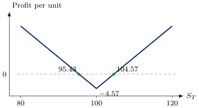
Figure 1. For the initial quote, a long straddle’s option payoff less its 4.5743 premium breaks even near 95.43 and 104.57. The stock-and-cash account below adds the gains and costs of maintaining its delta hedge.
2. Stock and cash accounting
At observation times \(t_0,\ldots, t_M=T\), let \(h_k\) be shares held over \([t_k, t_{k+1})\). The baseline target is
\[\begin{equation} h_k=-u\Delta_V(t_k, S_k;\sigma_Q). \label{eq:hedge} \end{equation}\]
This target uses the stock price observed at \(t_k\) and the option’s remaining time. The position is held until the next observation. As stock moves, option delta changes and the combined book acquires stock sensitivity between hedge times. A later rebalance changes inventory and cash at the then-current price.
Let \(h_{-1}=0\). If stock trading costs a fraction \(c\) of absolute traded notional, the cash update at \(t_k\) is
\[\begin{equation} B_k^+=B_k^--(h_k-h_{k-1})S_k-c|h_k-h_{k-1}|S_k. \label{eq:cash} \end{equation}\]
Buying shares uses cash; selling shares receives cash. The fee has the same negative sign for either trade direction. Start with \(B_0^-=-uV_0\). At expiry, liquidate the remaining shares, charge the declared terminal fee \(c_T\), and receive the signed option payoff \(uZ(S_T)\). At zero interest the resulting profit is exactly
\[\begin{align} \Pi={}&u[Z(S_T)-V_0]+\sum_{k=0}^{M-1}h_k(S_{k+1}-S_k)\nonumber\\ &-c\sum_{k=0}^{M-1}|h_k-h_{k-1}|S_k-c_T|h_{M-1}|S_T. \label{eq:pnl} \end{align}\]
The cash account charges the opening hedge as well as every subsequent rebalance and terminal liquidation. The cash balance can fall below zero during the strategy; borrowing at the study’s zero rate funds that balance.
On the same stock path, reversing \(u\) also reverses the frictionless target holdings. With zero fees, Equation (4) gives \(\Pi_{+u}=-\Pi_{-u}\). With proportional fees, both sides pay execution costs:
\[\Pi_{+u}+\Pi_{-u}=-(F_{+u}+F_{-u}).\]
We charge each actual net stock trade. If the call and put were instead hedged and executed separately, fees would apply to each leg’s stock trades. These arrangements can produce different costs because netting changes the amount of stock that reaches the market.
A call-plus-put basket and one straddle have the same financial profit when their aggregate payoff, initial price, hedge opportunities, inventory and execution rules match. Grouping those cashflows under one contract label or two preserves the result. Existing Volt tests verify this equivalence through P&L, risk and parameter gradients.
3. Gamma, variance and time decay
The physical stock model used in this experiment is
\[\begin{equation} dS_t=\sigma_P S_t\, dW_t^P. \label{eq:physical} \end{equation}\]
It has zero stock drift. Its constant parameter \(\sigma_P\) controls the simulated movement. The option is quoted and hedged using a separate constant \(\sigma_Q\) in the Black–Scholes formula [2]. A market option price could be converted into such an implied volatility by inversion. Here the quote volatility is specified directly so that the mechanism can be isolated. The hedge continues to use \(\sigma_Q\) even when the simulator uses a different \(\sigma_P\).
A realized variance statistic is a property of an observed path and sampling grid:
\[\widehat{\sigma}_{\rm RV}^{\, 2}=\frac 1T \sum_k\left[\log(S_{k+1}/S_k)\right]^2.\]
It varies across finite paths even when \(\sigma_P\) is constant. The report keeps fine-grid realized variance separate from its coarser hedge-grid counterpart. A parameter describing the distribution, an observed path statistic and a volatility implied by a quote should therefore be named separately in both code and analysis.
Write the option mark change over one interval as
\[\begin{equation} \Delta V_k=\Delta_k\Delta S_k+\Theta_k\Delta t +\tfrac 12\Gamma_k(\Delta S_k)^2+R_k. \label{eq:taylor} \end{equation}\]
The term \(R_k\) collects the part left after delta, theta and gamma: higher spot orders, time curvature and spot–time cross terms. We calculate it by repricing the option at the next observation and subtracting the displayed local terms. That lets us see how well the approximation explains each actual interval.
Combining Equations (4) and (6) gives the exact reported attribution
\[\begin{align} \Pi={}&u\sum_k\Theta_k\Delta t +\tfrac u 2\sum_k\Gamma_k(\Delta S_k)^2 +u\sum_k R_k\nonumber\\ &+\sum_k(h_k+u\Delta_k)\Delta S_k-F. \label{eq:attribution} \end{align}\]
For the exact delta target in Equation (2), the inventory-tracking term is zero at each interval start. A no-trade band or an unhedged position has a nonzero tracking term. The same identity accommodates both.
For a smooth zero-carry Black–Scholes quote, the pricing equation implies
\[\Theta_Q+\tfrac 12\sigma_Q^2 S^2\Gamma_Q=0.\]
Under continuous stock hedging, Itô’s formula and Equation (5) then yield
\[\begin{equation} d\Pi_t=\tfrac u 2\Gamma_Q(t, S_t)S_t^2 (\sigma_P^2-\sigma_Q^2)\, dt \label{eq:variance} \end{equation}\]
before execution costs. This explains the appearance of squared volatility. For a long positive-gamma option, more realized quadratic variation increases the convexity contribution, while the price paid for that convexity enters through time decay. A straddle weights this variance difference by its changing \(\Gamma S^2\). A variance swap has a different exposure profile, constructed using a range of strikes [3]. Two paths can therefore have equal unweighted realized variance and different straddle profits: their large moves may occur at different levels of gamma.
At the study’s initial state, consider a one-unit stock rise and one calendar day of time passage. After the initial stock hedge, the local approximation is
\[\Theta_0/365+\tfrac 12\Gamma_0(1)^2 =-0.076217469+0.069548441=-0.006669029.\]
Full repricing at \(S=101\) with 29 days remaining gives a delta-hedged interval profit of \(-0.007043579\), leaving a residual of \(-0.000374551\). For a one-unit decline to 99, the same quadratic approximation applies, but full repricing gives \(-0.005573061\) and residual \(+0.001095967\). We chose the up and down moves to work through the pricing formula. Their different residuals show how direction and curvature affect the approximation. In the simulation, we reprice at every observation and retain that residual in the account.
4. Experiment and assumptions
The study holds \(S_0=K=100\), remaining maturity \(30/365\) years and quote volatility \(\sigma_Q=20\%\). It varies physical volatility over 10%, 20% and 35%; position over one long and one short unit; and stock fees over 0, 1 and 5 basis points of traded notional. The opening and terminal trades pay the same fee rate as intervening trades. Each of 18 configurations uses 65536 paths and hedges 30, 60 or 120 times over the option’s life. There are 54 delta-hedged frequency cases and 54 no-hedge controls.
The physical law is continuous, constant-volatility, zero-drift GBM. Interest, dividends and borrow charges are zero. Options are executed at the stated model price with zero option fees; stock trades carry symmetric proportional charges. Inventory can be fractional and cash can be negative. Applying it to a traded strategy would also require margin, execution impact, trading hours, changing quotes and an estimated return process.
The finest grid has 120 Brownian increments. A 30-step hedge reads every fourth fine observation; a 60-step hedge reads every second observation. Both use the same terminal stock as the 120-step hedge. Position sign and fees also reuse those paths. Actual fine-path hashes agree across all six position/fee configurations within each physical-volatility cohort. This reuse makes the comparisons paired: each physical-volatility cohort supplies one common set of market paths across signs, fees and hedge frequencies.
For this zero-drift physical model, an adapted stock hedge has zero expected mark gain. The physical expectation of the European payoff is available from the same closed-form payoff integral evaluated at \(\sigma_P\). Consequently,
\[\begin{equation} \mathbb{E}_P[\Pi+F]=u\bigl[V_{\rm BS}(\sigma_P)-V_{\rm BS}(\sigma_Q)\bigr]. \label{eq:mean} \end{equation}\]
This applies to the no-hedge control and to every tested hedge frequency. Hedging changes the distribution; the execution costs change its mean. For one long unit, the analytic pre-cost expectations are \(-2.286915651\), zero, and \(+3.428465070\) in the 10%, 20% and 35% physical cohorts respectively. The simulation evaluates these controls without using them to modify paths or retune the strategy.
5. Measured returns, costs and tail risk
| Physical vol. | Hedges | Mean long profit | Standard error | Loss CVaR\(_{95\%}\) | Mean turnover |
|---|---|---|---|---|---|
| 10% | 30 | \(-2.286017\) | 0.002621 | 3.583492 | 311.330 |
| 10% | 60 | \(-2.286262\) | 0.002436 | 3.456002 | 416.477 |
| 10% | 120 | \(-2.286124\) | 0.002333 | 3.368818 | 558.591 |
| 20% | 30 | \(-0.000153\) | 0.002785 | 1.512959 | 432.427 |
| 20% | 60 | \(-0.001118\) | 0.002000 | 1.100047 | 582.625 |
| 20% | 120 | \(-0.000421\) | 0.001426 | 0.798313 | 791.034 |
| 35% | 30 | 3.423298 | 0.008072 | \(-0.620092\) | 528.069 |
| 35% | 60 | 3.421503 | 0.007337 | \(-0.735018\) | 716.678 |
| 35% | 120 | 3.424572 | 0.006924 | \(-0.768735\) | 980.421 |
Table 1. Measured zero-fee delta-hedged results for one long straddle unit, initial quote 4.574301 and quote volatility 20%. Each row uses 65536 paths. Profit, loss CVaR and turnover are in currency units; turnover is total absolute stock notional including opening and liquidation. Rows within a physical cohort share the same underlying paths.
When physical and quote volatility both equal 20%, the analytic pre-cost mean is zero. At 120 hedges, the measured mean is \(-0.000421\) with standard error 0.001426. A normal approximation to uncertainty in this sample mean gives an interval of approximately \([-0.003216, 0.002375]\) using 1.96 standard errors. The result is compatible with the independent expectation. The interval describes sampling uncertainty in the average profit under this simulation law. Individual outcomes vary much more widely, as the following quantiles show.
The unhedged position on the same paths has mean 0.002268 and standard error 0.013568. Its 95% loss CVaR is 4.393949, compared with 0.798313 for the 120-step hedge. The long hedged position’s 1% profit quantile is \(-0.925462\), median \(-0.003058\) and 99% quantile 0.991598. The unhedged 1% quantile is \(-4.504636\). Hedging has substantially concentrated this distribution around zero.
Loss CVaR averages the worst 5% probability mass of \(L=-\Pi\). The implementation uses the required fraction of the last observation when the tail contains a fractional number of paths, following Rockafellar and Uryasev [5]. A negative loss CVaR means the average profit remains positive even in that sample’s worst tail. Future paths can still produce losses. The reported standard errors describe sample means; quantiles and CVaR are point estimates for this study.
More frequent hedging reduces sampling dispersion in the matched-volatility control. Its standard error falls from 0.002785 at 30 hedges to 0.001426 at 120 hedges, while the mean stock turnover rises from 432.427 to 791.034. Once a 5 bp fee is applied to every trade, the same inventory path costs 0.216213 at 30 hedges, 0.291313 at 60 and 0.395517 at 120.
At 120 hedges, the measured mean becomes \(-0.395938\). The difference from the zero-fee mean equals the mean execution cost, since the same paths and targets are used. The 95% loss CVaR rises to 1.285710. Relative to 30 hedges with the same fee, 120 hedges still has a smaller loss-tail average in this particular cohort, but a more negative mean. Those two criteria lead to different choices. A trader choosing the frequency would therefore need to specify how much mean profit to give up for the smaller loss tail.
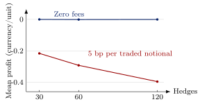
Figure 2. Measured mean profit for the long straddle at \(\sigma_P=\sigma_Q=20\%\). Points use identical fine stock paths; lines join only the three tested frequencies. Mean standard errors range from 0.001426 to 0.002785 without fees and from 0.001465 to 0.002744 with fees.
The turnover includes more than the visible rebalancing trades in the middle of the option’s life. For the matched-volatility 120-step case, initial hedge notional is 2.287151 and mean terminal liquidation notional is 94.214342. The remaining 694.532402 comes from intervening trades. At 5 bp these components cost approximately 0.001144, 0.047107 and 0.347266 respectively. Omitting terminal liquidation would materially understate the study’s reported execution cost. Transaction costs and revision frequency have long been linked in option replication theory [4]; the experiment exhibits that interaction using full cash accounting and actual net inventory changes.
For the 35% physical cohort quoted at 20%, the 120-step short straddle has mean profit \(-3.424572\), standard error 0.006924 and 95% loss CVaR 7.560771. Its median profit is \(-3.208861\), 1% quantile \(-8.147708\) and 5% quantile \(-6.639447\). The unhedged short position has loss CVaR 19.302638. The hedge reduces exposure to stock direction and its resulting tail dispersion, but the assumed movement is expensive for a seller of 20% volatility.
Conversely, in the 10% physical cohort, the 120-step short position earns a zero-fee sample mean 2.286124. The corresponding long position loses the same amount. At 5 bp both sides pay mean cost 0.279296, giving long mean \(-2.565420\) and short mean 2.006829. This is an arithmetic property of the specified physical-versus-quote difference and the common stock paths. Estimating such a difference in observed markets would require a forecast and executable option prices.
6. Greek attribution in measured paths
At 120 hedges and zero fees, the matched-volatility long straddle has mean theta contribution \(-2.284937906\), mean gamma contribution \(+2.284397997\) and mean full-repricing residual \(+0.000119043\). Their sum is \(-0.000420866\), the reported mean profit. The approximately 0.002689 delta contribution to the option mark is offset by the stock hedge. Time decay enters through the option values used in the attribution.
For the 10% physical cohort, mean theta is \(-3.038186820\) and mean gamma gain 0.759309823. The residual is \(-0.007247129\), giving mean profit \(-2.286124126\). For 35%, the corresponding terms are \(-1.664970086\), 5.097066198 and \(-0.007523848\), giving 3.424572264. Different stock paths spend different amounts of time near the strike, so their gamma and time-decay weights differ as well as their raw realized variances.
The left-point continuous-control integral from Equation (8) is approximately \(-2.278640115\), zero and 3.434000803 in the three cohorts at this frequency. Full-repricing profit includes discrete-interval effects and is the financial result used in the distribution and tail-risk tables.
A strategy using a volatility forecast or a moving quote surface would also incur gains and losses from revisions to those inputs. Those contributions would enter the same stock-and-cash account.
7. Validation and practical use
We checked the strategy through two routes: the profit formula and an independent cash-and-stock account. For every configuration and hedge frequency, eight selected paths were also replayed through Volt’s exact integer ledger. Those records include the option premium, each stock trade, fees and terminal settlement. The rounding rule for currency and shares is applied explicitly, so we can also measure its effect on the result.
All 864 ledger and rounding checks passed. Before rounding, the largest cash-account discrepancy was \(4.97\times10^{-14}\) currency units and the largest attribution discrepancy was \(3.55\times10^{-15}\). The largest observed rounding gap was \(5.96\times10^{-6}\), within its calculated allowance. Reversing the position and adding the two sides’ execution costs gave the expected zero sum to within \(3.33\times10^{-16}\) in the sample means. Across the zero-fee cases, the largest discrepancy from the independent expected profit in Equation (9) was 0.949 reported standard errors.
The matched-volatility position averages close to zero before fees; changing the simulated volatility changes the price of the payoff received; and stock turnover creates the observed execution cost. The application accepts the return volatility, quote volatility, position size, contract multiplier, hedge dates and fees separately, then returns the resulting profit distribution and its attribution. Processing market paths in batches controls the working memory needed for a larger run.
The same account can evaluate a fixed inventory band around the delta target. We retain the current stock position while it lies inside that band and trade to the nearest edge when it moves outside. The tables above use the exact delta target. To compare band widths, we would select a width on separate validation paths, save the choice, and measure its costs and risk on new paths.
References
[1] C. Bennett and M. A. Gil. Volatility Trading: Trading Volatility, Correlation, Term Structure and Skew. Santander Equity Derivatives, Madrid, 16 April 2012. Supplied research primer, especially pp.38–49 and 129–135. Back to text ↑
[2] F. Black and M. Scholes. The pricing of options and corporate liabilities. Journal of Political Economy, 81(3):637–654, 1973. https://doi.org/10.1086/260062. Back to text ↑
[3] K. Demeterfi, E. Derman, M. Kamal and J. Zou. More Than You Ever Wanted to Know About Volatility Swaps. Goldman Sachs Quantitative Strategies Research Notes, March 1999. Author’s archive: https://emanuelderman.com/more-than-you-ever-wanted-to-know-about-volatility-swaps-the-journal-of-der/. Back to text ↑
[4] H. E. Leland. Option pricing and replication with transactions costs. The Journal of Finance, 40(5):1283–1301, 1985. https://doi.org/10.1111/j.1540-6261.1985.tb02383.x. Back to text ↑
[5] R. T. Rockafellar and S. Uryasev. Conditional value-at-risk for general loss distributions. Journal of Banking & Finance, 26(7):1443–1471, 2002. https://doi.org/10.1016/S0378-4266(02)00271-6. Back to text ↑
This walkthrough is for research and educational purposes. It illustrates how strategynet.ai organizes signal evidence into factors and scenarios. It provides no recommendation, investment advice, or instruction to trade any security.
Back to Insights