
Options, Exercise and Learned Hedging: A Practical Primer
October 2026 · research@strategynet.ai · Web edition
Original PDF · LaTeX source · Option analytics and hedge-learning collection
An institution that sells an option receives money today and takes on a payment whose amount, and sometimes timing, depend on future markets. Stock positions can offset some of that exposure, while rebalancing incurs costs and early exercise can bring settlement forward. Understanding a learned hedge therefore begins with the contract, its financed trading account and the market conditions under which decisions are assessed. This primer develops the background needed to understand the option-pricing and hedge-learning applications in Volt and Jormungandr. We begin with a put option, follow its cash flows, introduce simulated market paths and distinguish forecasting from valuation. We then derive the holder’s exercise decision and the writer’s hedging problem, explain how training targets and derivatives are obtained, and connect the mathematics to the application interfaces. Worked calculations, compact diagrams and review questions accompany the discussion. Completed one-stock experiments provide a practical reference, while a reading guide leads into the original Deep Hedging and learned optimal stopping papers. The assumed background is basic algebra, functions and the idea of a derivative; probability, stochastic models and learning terminology are introduced as they become useful.
1. Options and contract terms
Suppose a fund owns shares and wants protection against a fall in their value. It buys a put: the right to sell a specified amount of stock at an agreed strike price, subject to the contract’s exercise terms. The seller, often called the writer, receives a premium for accepting the obligation. The fund now has protection, and the writer has a risk to manage.
Write \(S_t\) for the stock price at time \(t\), \(K\) for the strike and \(T\) for expiry. A cash-settled put pays \(g(S_T)=(K-S_T)^+\) at expiry, where \(x^+=\max(x,0)\). A call pays \((S_T-K)^+\). With \(K=100\), a put pays 10 if the stock finishes at 90 and zero if it finishes at 110. These payments are per underlying unit. The contract multiplier and position size turn them into the portfolio’s actual currency payments.
An option’s payoff describes the payment when it settles. Its value before settlement is the amount assigned to its remaining rights by a market quote or a valuation model. A put with the stock at 100 may be valuable because the stock can fall before expiry. Its immediate exercise payment is currently zero. Time, uncertainty, dividends and financing all enter the valuation [1].
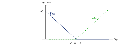
Exercise rights determine when the holder can take the payment. A European option permits exercise at expiry. A Bermudan option specifies a finite set of dates. An American option permits exercise through its contractual interval. In numerical work, increasingly frequent exercise dates can approximate continuous exercise. Physical settlement also specifies delivery of stock and strike cash; our worked learning examples use the economically specified cash payment.
The holder and writer have separate decisions. The holder chooses when to exercise. The writer chooses what to hold while the obligation is alive. A stock purchase can offset a short call’s exposure to a rise in price; a stock short can offset a short put’s exposure to a fall. Rebalancing costs money, so the useful hedge balances protection and execution costs. The exercise rule determines when that trading process ends.
We will follow a one-share put throughout. Illustrative calculations use explicitly chosen prices and payments. The measured training results appear in Section 8, where the model, units and sample sizes are stated.
2. Financing, units and settlement
A hedge is a financed portfolio. If a writer receives premium \(p\) and chooses \(h_0\) stock units at price \(S_0\), its cash balance becomes
\[b_0=p-h_0S_0-\lambda S_0|h_0|,\]
where \(\lambda\) is a proportional stock trading fee. A negative \(h_0\) is a stock short and raises cash when opened. Negative cash represents borrowing. At the next date, cash earns or pays interest and the stock is marked at its new price. The combined value is the money available to meet the liability.
Let \(b_n\) be cash after trading at date \(t_n\), and let \(D_{n+1}\) be a cash dividend per share paid at the next date. With constant annual funding rate \(r\) and interval \(\Delta t_n=t_{n+1}-t_n\), the pre-trade wealth on arrival, for a continuing contract with \(S_{n+1}\) measured ex-dividend, is
\[w_{n+1}^{-}=b_ne^{r\Delta t_n}+h_n(S_{n+1}+D_{n+1}).\]
Choosing new holdings \(h_{n+1}\) then leaves
\[b_{n+1}=w_{n+1}^{-}-h_{n+1}S_{n+1} -\lambda S_{n+1}|h_{n+1}-h_n|.\]
This formula pays for the inventory adjustment and its fee. It describes a self-financing hedge: after the initial premium, trades use the existing stock and cash account. More elaborate funding arrangements can supply different rates or explicit borrowing constraints.
For a concrete one-period calculation, sell a put for 6 with stock at 100, short 0.4 shares, and charge a 0.1% stock fee. Opening cash is \(6+40-0.04=45.96\). Suppose the stock subsequently reaches 90, cash grows by 1.001, and the put pays 10. Closing the stock short costs 36 and its closing fee is 0.036. The remaining cash is
\[45.96\times1.001-36-0.036-10=-0.03004.\]
Without the stock trade, the corresponding result is \(6\times1.001-10=-3.994\). The hedge offsets most of this particular loss. Another stock outcome produces a different result; the policy will be assessed across many paths.
If exercise occurs at time \(\tau<T\), the account closes its hedge there, pays the contract and keeps the remaining cash invested until \(T\). Reporting all path profits in currency at this common final date makes early and late settlements comparable. At constant rates, discounted profit is the final profit multiplied by \(e^{-rT}\). A study must say which convention its loss uses.
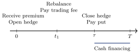
Contract units deserve the same attention as the model. If a put is quoted at 6 per share and its multiplier is 100, one contract costs 600. A model delta of \(-0.4\) means \(-40\) shares for that contract’s option exposure. For a writer hedging the short put, holding those \(-40\) shares offsets its positive stock-price sensitivity. Fees follow the actual shares traded. Applying the multiplier at both the payoff producer and the learner would scale the obligation twice.
Settlement timing also matters around dividends. If the exercise opportunity comes just before a cash dividend, the holder observes the pre-dividend stock price. A continuing stock position receives the dividend and moves to the ex-dividend mark. A hedge closed before that event receives the appropriate pre-dividend proceeds. Volt’s dated scenario producer records this ordering with its settlement and income arrays.
3. Probability and valuation
The future stock price is uncertain. A scenario specifies one possible sequence of prices, dividends and other observations. A random variable is a number determined by that uncertain future, such as the put’s payment. An expectation \(\mathbb{E}[X]\) averages a random variable \(X\) using its probability law. For two equally likely payments of zero and 10, the expectation is 5.
Expectations conditional on current observations are especially useful. \(\mathbb{E}[X\mid S_t=s]\) asks for the average future outcome among situations with that current stock state. A continuation-value model estimates this average payment from waiting. Its output changes with the information available now. A decision at date \(t\) uses observations up to that date, which we denote by \(\mathcal F_t\). This growing information set is called a filtration. It is the mathematical expression of observing the market as time passes.
Dispersion describes what an average leaves out. Variance is \(\operatorname{Var}(X)=\mathbb{E}[(X-\mathbb{E}[X])^2]\), and its square root is the standard deviation. Covariance measures how two variables move together; correlation rescales covariance by their standard deviations. A return generator for several stocks must describe these joint movements. Drawing every stock independently would impose zero dependence whether or not the intended model has that property.
We use two probability laws for different purposes. The physical law, \(\mathbb{P}\), models actual return outcomes and is used for forecasting and real-world risk assessment. A risk-neutral law, \(\mathbb{Q}\), is a pricing construction consistent with the selected tradable assets and financing assumptions. In the frictionless models used here, discounted gains including dividends are martingales under \(\mathbb{Q}\): their expected next value, conditional on current information, equals their current value.
For a European payment \(Z\) and deterministic rates, its model value is
\[V_t=\mathbb{E}^{\mathbb{Q}}[e^{-r(T-t)}Z\mid\mathcal F_t].\]
The exponential discounts future currency back to date \(t\). A stock’s physical expected return can include a risk premium or predictive signal. Under the GBM pricing specification, its ex-dividend drift becomes \(r-q\), where \(q\) is the continuous dividend yield. That change in probability law supplies the appropriate pricing expectation; the forecast retains its separate role.
This distinction becomes practical when we add factors. A factor model might forecast a stock rise under \(\mathbb{P}\). The writer can then benefit from retaining directional exposure, depending on its risk preference. A pricing calculation still needs coherent \(\mathbb{Q}\) dynamics or observed option marks. In a market with transaction costs and incomplete hedges, preferences and execution conditions also influence acceptable prices and positions. Our controlled pricing tests state a particular frictionless pricing model before evaluating trading costs.
A Monte Carlo calculation replaces an expectation by an average over simulated paths. For independent path outcomes \(X_1,\ldots,X_N\), define
\[\bar X=\frac1N\sum_{i=1}^N X_i,\qquad \operatorname{SE}(\bar X)=\frac{s_X}{\sqrt N},\]
where \(s_X\) is their sample standard deviation. Under the usual finite-variance central-limit approximation, \(\bar X\pm1.96\operatorname{SE}\) gives a 95% interval for the expectation. Four times as many independent paths roughly halves the standard error. Simulation bias, parameter uncertainty and model error require additional checks beyond that sampling interval.
When comparing two hedges, evaluate both on the same paths. The difference on each path then provides a paired observation, often giving a more precise comparison than two unrelated samples. Training paths improve the model; validation paths select its settings or checkpoint; fresh assessment paths measure the selected policy. Keeping these roles separate makes the final comparison useful. Repeatedly choosing policies using the assessment outcomes would turn that cohort into another selection dataset.
4. Market models, prices and Greeks
A stock model specifies how scenarios evolve. The simplest model used in our examples is geometric Brownian motion, or GBM:
\[dS_t=\mu S_t\,dt+\sigma S_t\,dW_t.\]
The parameter \(\mu\) is proportional drift, \(\sigma\) is annualized volatility when time is measured in years, and \(W_t\) is Brownian motion. A Brownian increment over an interval of length \(\Delta t\) is Gaussian with mean zero and variance \(\Delta t\), independently of earlier increments. The symbol \(dW_t\) represents that stochastic change in the continuous-time equation. The model assumes continuous positive stock paths and constant volatility.
GBM has an exact transition over a time interval:
\[S_{t+\Delta t}=S_t\exp\!\left[ (\mu-\tfrac12\sigma^2)\Delta t+\sigma\sqrt{\Delta t}\,Z\right], \quad Z\sim N(0,1).\]
Here \(N(0,1)\) denotes a standard normal draw. The \(-\sigma^2/2\) term follows from the stochastic change of variables for \(\log S\). Under the pricing law, \(\mu=r-q\). With several stocks, correlated Gaussian draws specify their joint Brownian increments. Exact GBM transitions remove time-stepping error for the stock at the simulated dates. The exercise and hedge calendars still determine which decisions are available.
Under GBM with constant volatility, rates and yield, the European call has an analytic value. For \(\sigma>0\) and remaining maturity \(\tau=T-t>0\),
\[\begin{aligned} C&=Se^{-q\tau}\Phi(d_1)-Ke^{-r\tau}\Phi(d_2),\\ d_1&=\frac{\log(S/K)+(r-q+\sigma^2/2)\tau}{\sigma\sqrt\tau},\qquad d_2=d_1-\sigma\sqrt\tau. \end{aligned}\]
\(\Phi(z)\) is the probability that a standard normal variable is at most \(z\). The formula assumes frictionless trading and the declared continuous GBM model. The corresponding European put is \(P=C-Se^{-q\tau}+Ke^{-r\tau}\), the put–call parity relation. It follows by comparing portfolios with the same terminal payments. Call delta is \(e^{-q\tau}\Phi(d_1)\); put delta subtracts \(e^{-q\tau}\). These analytic quantities supply useful numerical controls. The early-exercise problem adds the right to settle before the formula’s terminal date.
Heston gives volatility its own changing state. Write \(v_t\) for instantaneous variance. A common pricing specification is
\[\begin{aligned} dS_t&=(r-q)S_t\,dt+\sqrt{v_t}S_t\,dW_t^S,\\ dv_t&=\kappa(\theta-v_t)\,dt+\xi\sqrt{v_t}\,dW_t^v,\\ d\langle W^S,W^v\rangle_t&=\rho\,dt. \end{aligned}\]
For scale, volatility 20% corresponds to variance \(v=0.2^2=0.04\). The positive parameter \(\kappa\) controls mean reversion toward variance level \(\theta\); \(\xi\) controls variance fluctuations; \(\rho\) couples stock and variance shocks. This adds uncertainty that a stock-only hedge can leave exposed. Numerical simulation must also handle variance near zero and integration of variance between dates. Our European Heston studies and constant-volatility early-exercise studies use these distinct model specifications [5].
Once a model assigns option value \(V(S,\sigma,r,t)\), its derivatives describe local changes. Delta is \(\Delta=\partial V/\partial S\), gamma is \(\Gamma=\partial^2V/\partial S^2\), vega is \(\nu=\partial V/\partial\sigma\), rho is \(\partial V/\partial r\), and theta here is the derivative with respect to advancing calendar time. A short-horizon approximation is
\[\delta V\approx\Delta\,\delta S+ \tfrac12\Gamma(\delta S)^2+\nu\,\delta\sigma+ \frac{\partial V}{\partial r}\delta r+\Theta\,\delta t.\]
It is a local expansion with omitted cross terms and higher-order effects. A sufficiently large move calls for full repricing of the scenario.
The units determine how to read these numbers. Vega differentiated with respect to volatility as a decimal must be multiplied by 0.01 for a one-percentage-point volatility change. Annualized theta needs the declared day-count conversion for a daily display. Signed quantities and multipliers aggregate contract Greeks into portfolio Greeks. A delta near zero can coexist with substantial gamma or vega, so the portfolio’s response can still change rapidly as the market moves.
Implied volatility reverses the pricing calculation: choose volatility so the model price matches an observed option quote. Different strikes and expiries generally imply different values, producing the volatility grid commonly called a volatility surface. The fitted volatility is conditional on the pricing method, exercise rights, rates and dividends. Calibration errors or stale inputs can resemble trading opportunities in a cross-section. A practitioner therefore examines quote times and bid–ask prices alongside the calculated exposures. Quotes and open interest describe market observations and outstanding contracts; portfolio risk additionally requires signed positions. A sensitivity to initial Heston variance, \(\partial V/\partial v_0\), also carries different units from a derivative with respect to a scalar volatility. Each displayed Greek should identify the parameter being perturbed.
5. Exercise and dynamic programming
A holder of a put may exercise because the immediate payment is more useful than retaining the option. On a finite calendar, this becomes a sequence of comparisons. Let \(V_n(s)\) be the option value at date \(t_n\) when stock is \(s\). At expiry, \(V_N(s)=g(s)\). At an earlier exercise opportunity,
\[\begin{aligned} C_n(s)&=\mathbb{E}^{\mathbb{Q}}[e^{-r\Delta t_n}V_{n+1}(S_{n+1})\mid S_n=s],\\ V_n(s)&=\max\{g(s),C_n(s)\}. \end{aligned}\]
\(C_n\) is the continuation value. On dates where exercise is unavailable, the value is the continuation value alone. Starting from the known terminal payoff and moving backward is dynamic programming. Each earlier value uses the already computed later decisions.
A small tree makes the comparison concrete. Take a put with strike 100 and stock at 100. Exercise is allowed after either of two intervals. At each interval the stock multiplies by 1.2 or 0.8, while cash grows by a factor of 1.05. The pricing probability of an up move is chosen so the discounted stock has unchanged conditional expectation:
\[p_{\rm up}=\frac{1.05-0.8}{1.2-0.8}=\frac58.\]
At the low intermediate stock price of 80, exercise pays 20. Continuing gives
\[C_1(80)=\frac{(5/8)4+(3/8)36}{1.05}=15.2381.\]
The holder exercises. At stock 120, immediate payment is zero, whereas continuation is \([(5/8)0+(3/8)4]/1.05=1.4286\), so the holder waits. The initial Bermudan value is \([(5/8)1.4286+(3/8)20]/1.05=7.9932\). The terminal-only European value on the same tree is 6.2925. The additional exercise opportunity therefore contributes about 1.7007. The factor 1.05 is the chosen funding factor per interval; it is distinct from an annual continuously compounded rate.
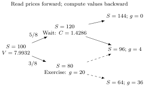
Trees and finite-difference grids approximate this recursion directly. The finite-difference method solves a pricing equation over stock and time; American exercise adds the condition that continuing value and immediate exercise satisfy an obstacle problem. Refining the spatial and temporal meshes checks numerical stability. As the number of underlying assets grows, a full grid requires many more points: \(m\) stock levels for each of \(d\) assets produce \(m^d\) combinations. This growth motivates simulation and learned continuation functions.
A stopping time \(\tau\) is a rule that decides to stop using the information available when it stops. For example, “exercise when immediate payment exceeds today’s estimated continuation” can be applied as the path unfolds. Selecting the most profitable exercise date after seeing the whole future would give the holder extra information. The numerical tests preserve this chronology both in exercise decisions and policy observations.
6. Neural policies and training objectives
A neural network is a parameterized function. Its weights, collected in \(\theta\), transform inputs through layers into an output. A hidden layer computes an affine transformation \(Ax+b\), then applies an activation such as \(\tanh\) or the rectified linear function \(\max(x,0)\). Changing the weights changes the function. Training chooses weights that improve a stated objective on the supplied examples.
For continuation regression, the input is today’s state. A future stopping rule, already selected during the backward calculation, supplies a discounted payment on each training path. Use the notation \(G_n=e^{-rt_n}g(S_n)\) and let \(\tau_{n+1}\) be that later rule. The regression fits a function \(c_\theta\) by minimizing
\[\frac1B\sum_{i=1}^{B} \left[c_\theta(S_n^{(i)})-G_{\tau_{n+1}^{(i)}}^{(i)}\right]^2.\]
The batch contains \(B\) paths. Here \(c_\theta\) estimates value discounted to time zero. Multiplying it by \(e^{rt_n}\) gives continuation in date-\(n\) currency, matching \(C_n\) in the earlier recursion. These targets are observed simulated payments; the network learns their conditional average. Its exercise decision compares \(G_n\) with \(c_\theta(S_n)\). Working backward makes the later rule available before fitting the current one. This is the continuation-regression approach used in the 2020 paper [8].
The 2019 direct approach instead learns an exercise decision. During training, a sigmoid output \(f_\theta(s)\) lies between zero and one. At each fitted date, it maximizes the average of
\[G_n f_\theta(S_n)+(1-f_\theta(S_n))G_{\tau_{n+1}}.\]
The objective rewards a larger immediate-payment weight in states where exercise is preferable, and a larger continuation weight where waiting is preferable. A threshold converts the selected function into a binary exercise rule. Both algorithms use future simulated outcomes to improve a rule that, when applied, observes only the current state [7].
A state is Markov when its current value determines the conditional law of the next state, given the model. Stock price supplies that state in GBM; Heston uses stock and variance together. When variance or a market regime is only partly observed, estimates and relevant history can enter the policy observation. A recurrent network can summarize that history through an internal state. The particular reset-LSTM engine in the completed stock-and-option study instead shares weights across dates and uses financial holdings and wealth to carry its specified history.
The writer’s network has a different output: target stock or instrument holdings. Write \(h_n=\pi_\theta(x_n,h_{n-1},w_n)\), where \(x_n\) contains the market observations, \(h_{n-1}\) contains previous holdings and \(w_n\) is wealth when that input is enabled. The account calculation converts all decisions into a final profit \(\Pi_T(\theta)\). Training can minimize
\[J(\theta)=\mathbb{E}[\Pi_T(\theta)^2].\]
The holder’s actual settlement, financing and transaction fees determine that profit. The episode begins with the received premium and zero hedge inventory. At each hedge date the action is the new vector of continuous holdings. The market simulator advances the observations, and the account advances cash and positions. The episode settles at the holder’s exercise date, then carries residual cash to the reporting horizon. For squared-loss training its terminal reward can be written \(-\Pi_T^2\). A CVaR objective depends on the loss distribution across episodes, which the batch calculation supplies. An analytic delta hedge can be a comparison strategy; the writer’s objective obtains its feedback from the simulated account.
Different risk preferences change the objective. Mean squared error penalizes both positive and negative departures from the chosen capital target. A downside squared loss uses \(\mathbb{E}[((-\Pi_T)^+)^2]\). For loss \(L=-\Pi_T\), a CVaR objective at confidence level \(\alpha\) can be written
\[\min_{\eta}\left\{\eta+ \frac{1}{1-\alpha}\mathbb{E}[(L-\eta)^+]\right\}.\]
CVaR averages the worst tail of losses; \(\eta\) is a fitted threshold. An entropic objective \((1/\gamma)\log\mathbb{E}[e^{\gamma L}]\), with risk-aversion parameter \(\gamma>0\), assigns increasing weight to large losses. The selected objective and premium determine what the learner is trying to improve. For example, \(\mathbb{E}[\Pi_T^2]=\operatorname{Var}(\Pi_T)+(\mathbb{E}[\Pi_T])^2\). Mean squared profit therefore measures dispersion and the squared mean departure from the chosen zero-residual target. Its units are currency squared; positive average profit is a separate reported statistic.
This is a sequential control problem: state, action, transition and eventual outcome. Reinforcement learning studies how to choose actions from such experience [10]. Our writer uses a differentiable simulator and optimizes complete paths, propagating derivatives through the trading account. The continuation learner uses regression targets, and the direct holder optimizes a stopping reward. Other Jormungandr policy engines can implement actor–critic or value-based RL algorithms. The method name in a study should identify which of these calculations produced its decisions.
A trained policy is a function of its supplied observations. A new stock price calls for a new evaluation of that function. The policy also carries training assumptions about liability, market law, horizon, costs and units. A policy intended to serve arbitrary portfolios needs those portfolio characteristics represented in its inputs and training distribution. Two portfolios with identical pathwise payments, initial capital, market law, risk objective and admissible hedging/execution terms share the same economic objective; matching their current Greeks alone provides a local comparison of exposure.
7. Automatic differentiation
Training needs to know how changing a weight changes the objective. A derivative answers that local question. Automatic differentiation, or AD, applies the chain rule to the actual sequence of numerical operations. Reverse mode is also called adjoint algorithmic differentiation, or AAD; neural-network backpropagation uses the same principle [9].
Consider the small calculation \(a=wx\), \(b=\tanh(a)\) and \(\ell=(b-y)^2\). Here \(x\) is an observed input, \(w\) is a weight and \(y\) is a target. The chain rule gives
\[\frac{\partial\ell}{\partial w} =2(b-y)(1-b^2)x.\]
For a large network, the program applies the same local rules through many operations. An optimizer such as Adam uses the resulting gradients, together with running first and second moments, to update the weights. Learning rate, normalization and the units of inputs influence the numerical trajectory.

A pricing sensitivity and a training gradient differ in what is varied. For delta, the input being differentiated is the stock price; model parameters and the contract’s valuation convention are held as specified. For a writer update, the differentiated inputs are policy weights. The same AD tooling can serve both tasks, provided the intended inputs remain connected to the calculation graph.
In forward mode, derivatives travel with the evaluated quantities. This is useful for a small number of input directions or selected higher-order quantities. Reverse mode propagates derivatives back from a scalar output to many inputs and usually retains intermediate values, or recomputes them, for that backward calculation. Those saved values contribute to memory use. A directional finite difference, obtained by perturbing an input and re-evaluating, supplies an independent numerical check on a derivative.
Financial functions include kinks. The put payoff changes slope at its strike; a proportional cost uses an absolute value; an exercise decision changes a branch. The estimator must respect that structure. Differentiating a sample path payoff can estimate certain sensitivities under appropriate regularity, while a second derivative of the same sampled kink needs additional treatment. For example, write a GBM terminal stock as \(S_T=S_0A\) with random multiplier \(A\). The put payment \((K-S_0A)^+\) is piecewise linear in \(S_0\), so its ordinary second derivative is zero away from the kink on each path. The expected option value can nevertheless have positive gamma. A suitable sensitivity estimator accounts for how probability mass near the strike changes with \(S_0\). Volt checks its supported gamma estimators separately. The learned holder is held fixed during the writer’s stopped-account training, and the account removes later policy actions after settlement.
A reliable training calculation also checks its scale. Stock holdings may be fractions, while another hedge instrument may require thousands of quoted units. Explicit input transforms and action scales can improve optimization while preserving the converted economic holdings. A good comparison restores all results to their declared financial units before comparing profits, fees and exposures. Our Heston studies show that these implementation choices can materially affect the fitted policy.
8. Validation and completed experiments
A policy’s training loss says how it performed on the paths used to improve it. The practical question is how its selected version behaves on different paths from the intended application law. We assess profit distributions, loss objectives, trading costs and comparison hedges on common fresh paths. An independent cash calculation checks the financial arithmetic, and separate derivative tests check that optimization receives the intended gradient.
Valuation of a learned holder offers another useful check. Under \(\mathbb{Q}\), its expected discounted exercise payment is a lower value relative to the best admissible exercise rule. A Monte Carlo average estimates that expectation with sampling uncertainty. An upper-value construction uses a martingale \(M_n\), starting at zero, to form
\[U=\mathbb{E}^{\mathbb{Q}}\!\left[\max_{n\text{ allowed}}(G_n-M_n)\right].\]
The martingale has zero expected gain when sampled at any allowed stopping time under the stated finite-horizon assumptions. Taking the maximum over allowed dates then makes this expectation at least the optimal stopping value.
Our initial estimator builds increments from a selected time-zero-discounted value approximation \(v_{n+1}\) and independent conditional simulations:
\[\delta M_{n+1}=v_{n+1}(S_{n+1})- \frac1K\sum_{k=1}^{K}v_{n+1}(\widetilde S_{n+1}^{(k)}).\]
Both terms have the same conditional mean given the current state. The fresh conditional children and the next outer stock draw preserve the martingale property with the stated information ordering. The papers describe a policy-tail construction; our continuation-proxy estimator supplies a separately identified alternative. More inner draws can reduce its extra simulation noise. The upper sample average has uncertainty too, so the report includes intervals around both expectations.
Volt’s numerical pricing engine supports American exercise through a finite-difference obstacle calculation, alongside European and dated Bermudan rights. Its tests include tree and QuantLib comparisons, dated cash dividends and mesh refinements. The learning results below use specified Bermudan dates. Their holder decisions, prices and hedge errors are evaluated under those calendars; refining the exercise dates provides a route toward continuous exercise. The pricing and learning guides document the separate interfaces [14].
Our one-stock application uses a put with spot and strike 100, 20% GBM volatility and 5% interest over one year. Two experiment calendars answer different questions. In the writer study, exercise is quarterly and hedging is monthly. Three seeds per cost setting each train for 3,000 updates using 16,384 training and 4,096 validation paths. The six selected policies are then compared on 16,384 fresh common paths.
| Strategy | Zero stock fees | 10 bp stock fees |
|---|---|---|
| Learned writer | 4.013 | 4.079 |
| Numerical delta | 3.935 | 3.984 |
| Selected stock band | 3.937 | 3.986 |
| Unhedged | 61.443 | 61.443 |
Table 1. Mean squared terminal-bank loss in currency squared for one underlying unit. One basis point is 0.01%; 10 bp is a fee fraction of 0.001 of traded notional. Learned entries average three selected policies.
The learned writer removes about 93% of unhedged squared loss. Numerical delta retains an advantage of about 2% of its own squared loss at this budget. The matching comparison intervals and all cash-account audits are given in the application paper. These values describe the stated synthetic model, contract, capital and execution assumptions.
The holder study permits exercise on all twelve monthly dates. It trains three seeds for each learned-stopping method, then evaluates discounted payments on 65,536 fresh paths. Payment estimates range from 5.952 to 5.983; the alternate upper estimates range from 6.262 to 6.292 using 4,096 outer paths and 64 conditional children per step. All six asymptotic 95% price enclosures contain the matching finite-difference value of 6.0428. The approximately 0.3 estimator gap measures remaining numerical room in this particular comparison.
The separate 2020 interval-hedge calculation learns how to hedge changes in approximate continuation values from one exercise date to the next. Three selected hedges have discounted-error MSEs of 3.986–4.116 on 32,768 additional paths, versus 54.57–58.60 for cash alone at their declared initial capital. The full writer and interval methods use different targets, financing representations and assessment cohorts, so their reports identify those conventions. The papers’ published multidimensional max-call experiments provide the next replication benchmark.
9. Portfolios and factor models
A portfolio adds many payments and overlapping risks. For a terminal-only book, its liability can be written \(Z=\sum_j n_jm_jg_j\), where \(n_j\) is signed liability quantity, positive for a payment owed by the writer, and \(m_j\) is its multiplier. Multiple exercise dates require that same aggregation at the actual settlement dates. The hedge policy can choose a vector of instrument holdings, and the cash account adds the gains and costs of each instrument.
A factor model describes shared movements across assets. One useful return representation is
\[r_{n+1}=\mu_n+B_n f_{n+1}+\varepsilon_{n+1}.\]
Here \(r_{n+1}\) is a vector of returns, \(\mu_n\) is their conditional mean, \(B_n\) is a loading matrix, \(f_{n+1}\) is a factor shock and \(\varepsilon_{n+1}\) is an idiosyncratic residual. Factor shocks and residuals have conditional mean zero here; any predictable means enter \(\mu_n\). A specified shock law and residual law turn the representation into a return generator. With log returns, prices evolve as \(S_{n+1}^i=S_n^i\exp(r_{n+1}^i)\), preserving positive prices. Simple returns instead require \(S_{n+1}^i=S_n^i(1+r_{n+1}^i)\) and admissible return support.
Principal component analysis, or PCA, finds orthogonal directions that explain sample variation [12]. For a return covariance estimate \(\Sigma\), its eigenvectors supply these directions and its eigenvalues give their variances. Retaining a few components compresses shared covariance. Generative use additionally specifies how shocks evolve, how residuals behave and how estimates update. Forecasting the conditional mean requires a further predictive model and an assessment of its uncertainty.
There are several research choices before attaching factors to a hedge. An economically named sector exposure, a PCA return component and a forecast signal represent different information. Their definitions, observation times, estimation windows and response to regime changes need to be specified. Option observations add implied volatility, skew and term structure, with liquidity and quote quality influencing the cross-section. A factor formed from Greeks also depends on each contract’s pricing conventions and units.
These quantities can also organize a live risk view. If \(b_{ik}\) is stock \(i\)’s loading on a small dimensionless factor return shock \(f_k\), its approximate stock-price change is \(S_i b_{ik}f_k\). For signed option units \(u_j\), positive for long positions, a first-order portfolio exposure to that factor is
\[A_k=\sum_j u_j\Delta_j S_{i(j)}b_{i(j)k},\]
where \(i(j)\) identifies contract \(j\)’s underlying. The linear price response is approximately \(A_k f_k\). Volatility factors add vega times their own volatility loadings, with consistent decimal or percentage-point units. Gamma contributes curvature. This gives stock, sector and factor views of the same option book, provided its positions and model conventions are known.
The intended experiment keeps the liability, paths, costs and assessment cohort aligned while comparing a hedge-only policy, a signal-trading policy and a combined policy. This reveals which gains come from protecting the liability and which depend on predicted returns. The signal law belongs to \(\mathbb{P}\); coherent option valuation still needs its pricing specification. Research on removing predictable drift from hedge training gives a related way to study this distinction [11].
Factor research therefore precedes the empirical combination. We will examine what existing models estimate, how to generate admissible joint paths, and which forecasts remain useful on data observed strictly after fitting. The published max-call benchmark first gives us a common multi-asset pricing and exercise reference under a fully declared model.
10. Applications and computational execution
The financial equations become an application through a few connected tools. Volt holds contract and portfolio definitions, generates or accepts scenarios, calculates prices and Greeks, and evaluates the hedge account. Burn supplies tensor operations, automatic differentiation and optimization. CubeCL supports GPU execution beneath the selected backend. Jormungandr supervises a persistent learner and supplies its HTTP lifecycle, dataset and inference operations. Hypercube publishes dated market and risk records for analytical applications. The implementation uses the backends and precision supported by its pinned build; the upstream Burn documentation explains the underlying architecture [13].
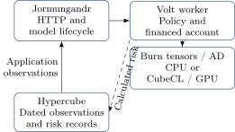
A GPU performs many related arithmetic operations in parallel. A batch of paths becomes matrices and vectors: a tensor is simply an array with a specified shape and data type. For example, stock marks have dimensions \([\text{path},\text{date},\text{instrument}]\). Keeping tensors resident on the device lets several calculations reuse them before transferring results back to the application. A Rust array uploaded through an API may involve allocation and copying even on a machine with physically shared memory; the selected tensor interface defines ownership and synchronization.
Memory budgeting means estimating the peak storage needed before admitting a workload. With \(B\) paths, \(L\) dates, \(d\) instruments and \(s\) bytes per scalar, marks alone use approximately \(BLds\) bytes. At \(B=100{,}000\), \(L=31\), \(d=10\) and f32 storage, that is 124 million bytes, about 118 MiB. Features, activations, gradients, optimizer moments, temporary kernels and transactional copies add to this amount. Streaming smaller batches keeps the study’s total path count independent of its resident batch size.
GPUs help when enough parallel work amortizes dispatch, synchronization and transfer time. A small date-specific network can run faster on a CPU. Fusion can combine compatible tensor operations into fewer kernels and reduce intermediate traffic. Floating-point precision and reduction order also affect numerical results, especially when subtracting nearby values. We measure the actual configured training or pricing calculation, with its accuracy checks, to choose a device.
Three CPU commands demonstrate the learning application:
cargo build --release -p volt-compute --bin deep_stopping --bin bermudan_market --bin native_learner
python3 examples/deep_stopping.py --output /tmp/volt-stopping-example
python3 examples/bermudan_learning.py --output /tmp/volt-bermudan-example
The first example fits a holder and an interval hedge, then estimates valuation and hedging results on independent paths. The second fits a writer against a numerical holder, selects its checkpoint on validation and compares it with a financed delta control on fresh paths. Each retains the inputs and results needed to inspect the complete sequence. The default examples use small, bounded budgets; the completed studies above have their own fixed protocols.
Through Jormungandr, an application creates a native model, registers dataset partitions, uploads a scenario batch, requests a versioned update, evaluates held-out paths and retrieves a checkpoint or target holdings. The writer’s batch supplies stock marks, decision-time features and actual settlement indices and amounts. Optional income and initial-capital arrays make the financial convention explicit. Current observations and holdings then feed inference until the contract settles. The API guides provide exact request schemas and executable examples [14], [15].
11. Exercises and further reading
The following short checks connect the main ideas. They are useful before changing a market model or interpreting a training result.
-
A put with strike 100 expires at stock 92. For three contracts with multiplier 100, what is the payment? It is \(3\times100\times8=2{,}400\) to the holder. Premium and hedge gains determine the writer’s final profit.
-
A model vega is 24 per underlying unit for volatility expressed as a decimal. What is the approximate effect of a one-percentage-point increase on one long contract with multiplier 100? It is \(24\times0.01\times100=24\).
-
A portfolio’s Monte Carlo standard error is 0.04 using 10,000 independent paths. How many comparable paths target 0.02? Approximately 40,000, keeping the same distribution and estimator.
-
On an exercise date, a put’s immediate payment is 7 and its model continuation value is 6.5. What does the value-maximizing holder do? It exercises. The writer closes its hedge and settles according to the event order.
-
A factor model explains most historical covariance. What must be added to generate return scenarios? A shock distribution and evolution law, a residual model, the conditional-mean convention and a dated estimation rule.
-
A policy responds correctly to a new stock price. What determines whether it can handle a different portfolio? Its observations and training distribution must represent the relevant portfolio payments, quantities and contract terms.
For contract terms and everyday quotation conventions, begin with the Options Industry Council material [1], [2]. Then read the worked accounts in this primer and the Jormungandr application paper. Glasserman’s Monte Carlo Methods in Financial Engineering develops simulation, estimation and variance reduction; Shreve’s Stochastic Calculus for Finance II develops pricing measures and continuous-time models [3], [4].
Read the original Deep Hedging paper next for after-cost portfolio objectives and learned trading decisions [6]. Becker, Cheridito and Jentzen’s 2019 paper develops direct stopping, followed by their 2020 treatment of continuation regression, bounds and hedging [7], [8]. Baydin and colleagues explain AD and its relationship to backpropagation [9]. Sutton and Barto provide the wider sequential-learning framework [10]. Jolliffe and Cadima review PCA and its interpretation before the factor-model extensions [12]. The repository guides then connect these methods to the supplied APIs.
A useful progression is to reproduce the one-period cash arithmetic, run both small examples, inspect a saved exercise path and compare a selected hedge on fresh scenarios. From there, study the common multi-asset benchmark before introducing estimated factors and predictive signals. Each step adds a specific source of complexity while retaining calculations that can be checked.
References
[1] Options Industry Council. Options Pricing. Contract values and pricing inputs. https://www.optionseducation.org/optionsoverview/options-pricing. Back to text ↑
[2] Options Industry Council. Exercising Options. https://www.optionseducation.org/optionsoverview/exercising-options. Back to text ↑
[3] P. Glasserman. Monte Carlo Methods in Financial Engineering. Springer, 2003. https://doi.org/10.1007/978-0-387-21617-1. Back to text ↑
[4] S. E. Shreve. Stochastic Calculus for Finance II: Continuous-Time Models. Springer, 2004. https://link.springer.com/book/9780387401010. Back to text ↑
[5] S. L. Heston. A Closed-Form Solution for Options with Stochastic Volatility with Applications to Bond and Currency Options. Review of Financial Studies 6(2):327–343, 1993. https://doi.org/10.1093/rfs/6.2.327. Back to text ↑
[6] H. Buehler, L. Gonon, J. Teichmann and B. Wood. Deep Hedging. 2018. https://arxiv.org/abs/1802.03042. Back to text ↑
[7] S. Becker, P. Cheridito and A. Jentzen. Deep Optimal Stopping. JMLR 20(74):1–25, 2019. https://jmlr.org/papers/v20/18-232.html. Back to text ↑
[8] S. Becker, P. Cheridito and A. Jentzen. Pricing and hedging American-style options with deep learning. JRFM 13(7):158, 2020. https://arxiv.org/abs/1912.11060. Back to text ↑
[9] A. G. Baydin, B. A. Pearlmutter, A. A. Radul and J. M. Siskind. Automatic differentiation in machine learning: a survey. JMLR 18(153):1–43, 2018. https://arxiv.org/abs/1502.05767. Back to text ↑
[10] R. S. Sutton and A. G. Barto. Reinforcement Learning: An Introduction, second edition. MIT Press, 2018. https://mitpress.mit.edu/9780262039246/reinforcement-learning/. Back to text ↑
[11] H. Buehler, P. Murray, M. S. Pakkanen and B. Wood. Deep Hedging: Learning to Remove the Drift under Trading Frictions with Minimal Equivalent Near-Martingale Measures. 2021. https://arxiv.org/abs/2111.07844. Back to text ↑
[12] I. T. Jolliffe and J. Cadima. Principal component analysis: a review and recent developments. Philosophical Transactions A 374:20150202, 2016. https://pmc.ncbi.nlm.nih.gov/articles/PMC4792409/. Back to text ↑
[13] Burn project. Backend and automatic-differentiation documentation. https://burn.dev/books/burn/. Back to text ↑
[14] Volt. Exercise pricing, native hedge learner, Bermudan scenarios and learned stopping guides. https://github.com/ingvor-restrat/volt/blob/main/docs/exercise-pricing.md. https://github.com/ingvor-restrat/volt/blob/main/crates/volt-compute/docs-native-learner.md. https://github.com/ingvor-restrat/volt/blob/main/docs/bermudan-market.md. https://github.com/ingvor-restrat/volt/blob/main/crates/volt-compute/docs-deep-stopping.md. Back to text ↑
[15] Jormungandr. Native learner API and mathematical application tutorial. https://github.com/ingvor-restrat/jormungandr/blob/main/docs/native-learners.md. https://github.com/ingvor-restrat/jormungandr/tree/main/docs/latex/hedging. Back to text ↑
This walkthrough is for research and educational purposes. It illustrates how strategynet.ai organizes signal evidence into factors and scenarios. It provides no recommendation, investment advice, or instruction to trade any security.
Back to Insights