
Pricing and Risk Analytics with Volt: Applications, APIs and CPU/GPU Execution
October 2026 · research@strategynet.ai · Web edition
Original PDF · LaTeX source · Derivative portfolio risk
An options book can contain thousands of contracts whose values and hedge requirements change with each market update. A risk application needs to connect those observations to contract prices, portfolio exposures and the effects of possible stock or volatility moves. Volt provides batch valuation and sensitivity APIs, a quote-to-surface risk service and a persistent learner interface for hedging applications. We follow a small call-and-put book through those tools, explain the units returned by each calculation, and show how automatic differentiation and CPU/GPU execution support larger workloads. On an RTX 4090 test system, valuing 65,536 rows already held on the device takes 0.67 milliseconds on CUDA and 1.75 on CPU; a complete first-order Greek report with spot gamma takes 27.66 milliseconds on CUDA and 24.24 on CPU. The resident valuation benefits from CUDA; the complete Greek request runs faster on CPU at this size. Independent numerical controls cover Black–Scholes, shared-factor sensitivities, Monte Carlo estimators and Heston pricing.
1. Pricing and risk in an application
Consider a desk holding calls and puts on a stock. A new market observation changes the estimated value of those contracts and the positions needed to hedge them. The desk wants both numbers quickly. It also needs to understand what caused the change: a move in the stock price, a change in volatility, the passage of time, or a change in the model’s assumptions.
For a call with delta 0.55, a one-unit stock rise increases its value by about 0.55 per underlying unit. A trader who has sold the call can buy 0.55 shares to offset that first-order exposure. As the stock moves, delta changes; gamma measures that response. Vega describes the change in option value as the assumed volatility moves. These sensitivities form the book’s Greeks.
For 256 risk inputs, central differences require 512 portfolio repricings: one upward and one downward move for each input. Every added contract then adds work to each of those repricings. Automatic differentiation shares the price calculation across its input sensitivities, while a GPU can evaluate many contract rows in parallel. Volt exposes these calculations through interfaces that a batch process, a risk panel or a hedging application can call.
Figure 1 shows how the application request reaches its financial and numerical calculation, and where the resulting tensors live.
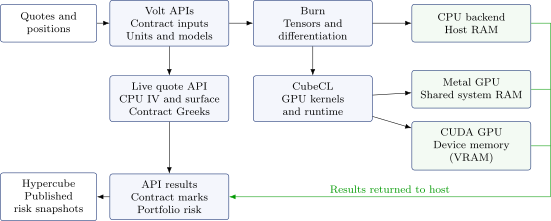
Figure 1. Volt connects the financial request to its numerical route. Burn manages tensors and derivatives; CubeCL supplies GPU execution. CPU data uses host RAM, Apple Metal resources use shared system RAM, and CUDA tensors use GPU memory. Completed portfolio results are published through Hypercube.
2. The request and result APIs
The application submits a contract book and an as-of market snapshot. The book supplies contract identity, signed quantity and multiplier; the snapshot supplies the underlying price, volatility, rates, dividend yield and observation time. The VoltValuationRequest interface checks those records and projects supported contracts into the numerical calculation [11]. The current valuation adapter accepts unexpired European calls and puts. Their exercise and settlement records remain attached to the contract.
Applications can use the native library calls or the supplied command-line runners. A valuation result contains contract marks and an aggregated book value. The sensitivity API adds delta, vega, rho, calendar theta and dividend-yield sensitivity; callers can request spot gamma as well. Per-contract outputs retain the input row identity, and the portfolio calculation applies the original signed quantities and multipliers. This lets a risk panel trace a large exposure back to its contributing positions.
| Application | Supplied calculation |
|---|---|
| Batch risk | Contract values, Greeks and signed portfolio totals |
| Scenario analysis | Revaluation under supported stock and volatility changes |
| Live option view | Quote-implied volatilities, fitted surface, book Greeks and scenarios |
| Hedge learning | Continuous holdings, financed cash flows, terminal risk and policy updates |
For an overnight risk report, the sensitivity runner can read a canonical portfolio request and write a summary together with one result per row:
aad_bench --volt-input book.json \
  --device cpu --precision f64 --gamma \
  --output risk.json \
  --greeks-output rows.jsonl
The same input can be submitted to a GPU-enabled build with the chosen device and precision. A planning request checks the calculation and estimates its working memory before opening the device. Larger books can be processed in chunks while retaining ordered contract results and stable portfolio sums.
The live option service accepts a complete quote-and-position frame through POST /api/quotes. It calculates bid, midpoint and ask implied volatilities, fits a surface, updates the book’s Greeks and revalues declared spot and volatility scenarios. A caller can read the latest result through GET /api/snapshot or subscribe to updates through GET /api/stream. Hypercube publishes the associated risk snapshot, which the web and terminal viewers consume. The current live analytics route runs on CPU; the tensor pricing and AAD interfaces provide the separate CPU/GPU calculation route shown in Figure 1.
A hedging application can also train a policy from complete scenario batches. Jormungandr provides the control API, while an optional persistent Volt/Burn worker retains the policy, optimizer and scenario tensors [12]. The policy chooses stock and option holdings. The worker carries those holdings through transaction costs, cash funding, dividend income and terminal liquidation, then differentiates the final risk objective with respect to the policy weights. Each update has an expected model version, and registered dataset partitions keep training, validation and test ranges separate. This learner interface supports the existing continuous MLP policy with previous-holdings feedback. The companion hedging article develops the learning problem and its experimental evidence.
3. Contract values and portfolio exposure
A European call gives its holder the right to buy at the agreed strike on expiry; a put gives the right to sell. Their expiry payoffs are \((S_T-K)^+\) and \((K-S_T)^+\), where \(x^+=\max(x,0)\). A pricing model estimates the current value of one option per underlying unit. The book tells us how many units are owned. For contract \(i\), write its model price as \(C_i\), signed quantity as \(n_i\), and contract multiplier as \(m_i\). The position weight is \(w_i=n_i m_i\), giving portfolio value
\[\begin{equation} V=\sum_{i=1}^{N} w_i C_i.\label{eq:portfolio} \end{equation}\]
That same weight applies to each of the contract’s per-unit Greeks. A short position contributes a negative weight. Its contract still describes the same payoff; the sign records which side of that payoff the book owns.
Take a European call and put on the same stock with
\[S=K=100,\quad T=0.5,\quad \sigma=0.20,\quad r=0.03,\quad q=0.01.\]
Here \(S\) is spot, \(K\) the strike, \(T\) the remaining years, \(\sigma\) annual volatility, \(r\) the continuously compounded rate and \(q\) the dividend yield. The example portfolio holds ten calls and is short four puts, each with multiplier 100. The Black–Scholes formula gives
| Per underlying unit | Call | Put |
|---|---|---|
| Price | 6.090127 | 5.100073 |
| Delta | 0.553457 | \(-0.441555\) |
| Vega per unit \(\sigma\) | 27.789495 | 27.789495 |
| Gamma | 0.0277895 | 0.0277895 |
The weights are 1000 and \(-400\), so
\[\begin{align*} V&=1000C-400P=4050.097918,\\ \Delta_V&=1000\Delta_C-400\Delta_P=730.079337,\\ \nu_V&=600\times27.789495=16673.696849,\\ \Gamma_V&=600\times0.0277895=16.673697. \end{align*}\]
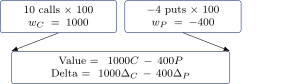
Figure 2. Quantities and multipliers give signed underlying units. The same weights carry each contract’s price and Greeks into the portfolio.
A volatility move from 20% to 21% is a change of 0.01 in \(\sigma\), making the first-order vega effect about 166.737 currency units. For a one-unit spot rise, delta and gamma give
\[\Delta V\approx\Delta_V\Delta S+\tfrac12\Gamma_V(\Delta S)^2 =738.416185.\]
In this calculation we hold volatility and the other model inputs fixed. A surface that moves with spot defines a further sensitivity, developed in the companion article on live option risk.
Rho is \(\partial V/\partial r\), so a one-basis-point rate move multiplies it by \(10^{-4}\). Calendar theta is \(-\partial V/\partial T\), because remaining time falls as the calendar advances. The adapter uses Actual/365 Fixed for maturity; its one-day linear theta approximation divides the annual value by 365. A book spanning several currencies would also need an explicit FX conversion rule before aggregation.
4. Automatic differentiation for Greeks
The Black–Scholes price of a European call is
\[\begin{align} C&=Se^{-qT}\Phi(d_1)-Ke^{-rT}\Phi(d_2),\label{eq:bs}\\ d_1&=\frac{\log(S/K)+(r-q+\sigma^2/2)T}{\sigma\sqrt T},\nonumber\\ d_2&=d_1-\sigma\sqrt T.\nonumber \end{align}\]
The normal cumulative distribution is \(\Phi\), with density \(\phi\). The put follows from \(P=C-Se^{-qT}+Ke^{-rT}\) [1]. For positive spot, strike, maturity and volatility, we can differentiate through the logarithm, square root, exponentials and normal probabilities.
Automatic differentiation applies the chain rule to these operations as the program runs [2]. Reverse mode starts from the final scalar and works back through the intermediate values. The sensitivity of the result to an intermediate value is called its adjoint. If \(z=f(x,y)\) and its adjoint is \(\bar z\), the local reverse step adds
\[\bar x\mathrel{+}=\bar z f_x,\qquad \bar y\mathrel{+}=\bar z f_y.\]
The additions allow an input used in several places to receive every contribution. For example, with \(a=\log S\), \(b=a^2\) and \(V=wb\), the reverse calculation starts at \(\bar V=1\) and gives
\[\bar b=w,\qquad \bar a=2a\bar b,\qquad \bar S=\bar a/S.\]
A larger pricing program repeats these same small steps. It retains or recomputes the intermediate values needed by each derivative rule, which explains the additional memory used during a reverse calculation.
For Black–Scholes the independent checks include
\[\Delta_C=e^{-qT}\Phi(d_1),\quad \nu_C=Se^{-qT}\phi(d_1)\sqrt T,\quad \Gamma_C=\frac{e^{-qT}\phi(d_1)}{S\sigma\sqrt T}.\]
We compare each computed Black–Scholes Greek with these analytic formulas, which establish its units and provide an independent accuracy check. When a pricing program contains more steps, we can apply the same local derivative rules throughout that program. Giles and Glasserman develop this approach for Monte Carlo risk [3].
For stocks exposed to common market factors, let \(x_j\) be a log-price shock and \(B_{ij}\) its loading on asset \(i\). Define
\[\begin{equation} S_i(x)=S_{i0}\exp\!\left(\sum_{j=1}^{D}B_{ij}x_j\right),\qquad V(x)=\sum_i w_iC_i(S_i(x)).\label{eq:factors} \end{equation}\]
Reversing that calculation gives all the factor sensitivities:
\[\begin{equation} \frac{\partial V}{\partial x_j} =\sum_i B_{ij}w_i\Delta_i S_i.\label{eq:factorgradient} \end{equation}\]
A unit loading with \(x_j=0.01\) produces approximately a 1% spot move. The loadings describe this risk experiment; a statistical scenario model would also supply a distribution for the factors and their dependence.
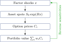
Figure 3. The forward calculation builds one portfolio value. The reverse calculation follows its dependence on every factor.
Central differences would reprice the book at \(x+he_j\) and \(x-he_j\) for each factor, requiring \(2D\) prices. Reverse mode shares the pricing work across all \(D\) derivatives. Forming the dense projection \(Bx\) and its reverse still costs on the order of \(ND\), and the program returns \(D\) results. This is the useful computational saving: expensive pricing work is reused across its inputs.
For Black–Scholes spot gamma, Volt carries three values through each operation: its value, first derivative and second derivative in the spot direction. Seeding spot with \((S,1,0)\) and constants with \((c,0,0)\) gives, for example,
\[(fg)''=f''g+2f'g'+fg'',\qquad (\log f)''=f''/f-(f'/f)^2.\]
Applying these rules through Equation (2) gives spot gamma directly. A change of coordinates adds its own curvature. In a one-factor log-price experiment, the corresponding second derivative is
\[\frac{\partial^2V}{\partial x^2} =\sum_i w_iB_i^2(\Gamma_i S_i^2+\Delta_i S_i).\]
The delta term follows from differentiating the exponential spot map twice.
A simulated payoff raises a different issue. Under risk-neutral geometric Brownian motion (GBM), a call price is the discounted expectation of \((S_T-K)^+\), with
\[S_T=S\exp\!\left((r-q-\tfrac12\sigma^2)T+\sigma\sqrt T Z\right), \qquad Z\sim N(0,1).\]
For each sampled path, the first derivative propagates through \(S_T\) and the payoff. The payoff’s slope changes at the strike, however, and its indicator is constant on either side. A second pathwise differentiation misses the probability mass crossing that strike as spot changes.
We account for that movement with a likelihood-ratio estimator, which weights each discounted payoff by
\[\begin{equation} W_\Gamma(Z)=\frac{Z^2-1}{S^2\sigma^2T} -\frac{Z}{S^2\sigma\sqrt T}.\label{eq:lrgamma} \end{equation}\]
This estimates the second derivative of the expected price [4]. Its sampling error is measured alongside the estimate. When using paired normal draws \((Z,-Z)\), each pair supplies one independent observation. For a portfolio, common draws also preserve covariance between its estimated position risks. A multi-asset market model supplies the economic dependence between assets.
5. GPU execution and memory
The implementation uses Burn for tensors and automatic differentiation, and CubeCL for accelerator execution [7], [8]. A tensor is an array with a shape, a number format and an execution device. These choices are explicit in a Volt session. The CPU path supports 32-bit and 64-bit floating point (f32 and f64), Metal supports the tested f32 path, and CUDA supports both. The session checks the requested combination before executing it.
Hypercube handles the publication side of the live application. It groups calculated prices and risks with their observation times and portfolio version into a coherent snapshot. The current live surface application calculates its IVs, fitted surface and Greeks through the CPU analytics route. Batched pricing and AAD requests use Burn’s tensor route, which can select CPU or GPU execution. Figure 1 shows where those routes sit in the application.
An application array is packed into the selected number format and uploaded into a device tensor. Kernel operations then use those tensors, and a readback returns the requested results to the host. Matrix shape is part of the request: an \(m\times k\) array multiplied by a \(k\times n\) array produces an \(m\times n\) result. Rectangular and odd-sized fixtures exercise the layouts and partially filled work tiles that arise in larger financial calculations.
On Apple Silicon, CPU and GPU share physical memory. Metal still assigns a storage mode to each resource and coordinates access to it [9]. The current tensor API handles that allocation and upload. The application retains its host inputs while the runtime manages the device resources. A discrete NVIDIA GPU adds a transfer between host memory and device memory. Reusing inputs on the device spreads this exchange cost over more calculations [10]. That reuse is called residency.
For one request, the elapsed time has several parts:
\[\begin{align*} t_{\rm job}={}&t_{\rm setup}+t_{\rm pack}+t_{\rm upload} +t_{\rm calculation}\\ &+t_{\rm synchronization}+t_{\rm readback}+t_{\rm aggregation}. \end{align*}\]
The first request may also initialize a device context and compile kernels. Enqueuing GPU work can return while the device is still calculating, so a completed-work timing includes the required synchronization.
Volt’s persistent valuation route uploads its inputs once and can apply supported uniform spot changes on the device. Each current AAD request builds its own derivative graph. These routes therefore have different reuse and storage costs, even when they start from the same option rows. The measurements below show the consequence: resident valuation benefits from CUDA at a tested size where a complete price-and-Greeks request remains faster on CPU.
For the current f32 first-order AAD workload, the memory planner allows 256 scalar graph slots, 512 bytes of staging and 48 bytes of returned values per row. At 65,536 rows these terms are 64 MiB, 32 MiB and 3 MiB, totaling 99 MiB before the other declared reserves and headroom. The graph term becomes 128 MiB at f64; a gamma calculation receives its own additional allowance. These estimates let the planner choose a batch size before allocating the work.
If that work exceeds the allowance, the calculation can proceed in row chunks. A portfolio sum combines the chunks in source order, and the shared-factor example combines each chunk’s \(D\)-component gradient in the same way. Smaller chunks reduce live memory and repeat more setup, calculation and readback work. We measured this tradeoff directly: for 1,024 positions and 256 factors on an Apple M3 using Metal f32, increasing the chunk from 32 to 1,024 rows raised sampled live allocation from about 38 KB to 1.10 MB while reducing elapsed time from roughly 112 ms to 6.1 ms. The aggregate gradient passed the same accuracy checks. These observations came from a host running other work.
The 99 MiB allowance above estimates array storage and derivative workspace. Allocator samples measure storage at a particular point during execution; process memory also includes host and runtime state. Caller-owned market data, compiler storage and other applications enter the deployment’s memory plan separately.
6. Heston pricing and numerical validation
Heston models variance as a process that evolves alongside the stock price [5]:
\[\begin{align*} dS_t&=(r-q)S_t\,dt+\sqrt{v_t}S_t\,dW_t^S,\\ dv_t&=\kappa(\vartheta-v_t)\,dt+\xi\sqrt{v_t}\,dW_t^v,\\ d\langle W^S,W^v\rangle_t&=\rho\,dt. \end{align*}\]
Variance \(v_t\) returns towards its long-run level \(\vartheta\) at speed \(\kappa\). The parameter \(\xi\) controls its random fluctuations, while \(\rho\) links those fluctuations to stock moves through the two Brownian drivers \(W^S\) and \(W^v\). The model’s characteristic function, the expectation of a complex exponential of log price, lets us calculate European option values through Fourier integrals.
The GPU evaluates those integrals on a fixed numerical grid. A Black–Scholes control variate improves the arithmetic: we add its known price and integrate the difference between the two characteristic functions. Heston’s dynamics continue to determine the result. Differentiating this calculation supplies sensitivities to the pricing inputs and variance parameters; Fourier spot derivatives also supply gamma.
Heston’s initial variance is \(v_0\), so \(C_{v_0}\) measures price per variance unit. If we choose to express \(v_0=\sigma_0^2\), the chain rule gives
\[\frac{\partial C}{\partial\sigma_0}=2\sigma_0 C_{v_0}.\]
The companion hedging paper uses these model sensitivities to construct its stock and variance-instrument comparison strategy.
Analytic Black–Scholes Greeks test the smooth pricing graph. Central repricing and the analytic factor expression in Equation (4) verify shared-factor sensitivities. Monte Carlo estimates are compared with analytic prices and Greeks using their sampling uncertainty. Heston has a separate CPU-f64 reference that adds integration points where the estimated error is larger, with explicit evaluation limits and a tail estimate within its stated parameter domain [6].
In central differences, a smaller bump reduces truncation error but increases subtraction roundoff, whose contribution scales roughly as \(\epsilon |V|/h\). We compare several bumps. For a Fourier integral, extra nodes improve accuracy within the chosen interval; extending the cutoff includes more of the tail and introduces more oscillations to resolve. We vary node count and cutoff separately. This is particularly useful near zero variance and short maturity, where the tail can be demanding.
An f64 derivative rule used a lower-precision reciprocal within the normal-CDF calculation. Direct Greek checks exposed the error, and expressing the constant operation through its reciprocal restored the expected accuracy. On CUDA, native special functions through the C++ backend and NVIDIA’s runtime CUDA compiler (NVRTC) supplied the precision required by these checks.
Dense matrix fixtures exposed reduced-precision multiplication in the selected CUDA route, despite the arrays being stored as f32. The supported CUDA matrix route uses strict multiplication, and small differentiable policy layers use bounded products and reductions. For portfolio totals, ordered compensated f64 sums preserve small residual exposures when large positive and negative positions nearly offset.
The numerical checks cover prices, first derivatives, spot gamma and shared factor sensitivities on the supported CPU, Metal and CUDA routes. Each route is checked against the corresponding independent formula, numerical reference or statistical estimate. The shared-factor checks cover 256 positions with 1, 4, 16, 64 and 256 inputs, using both analytic derivatives and central repricing. The supported precision is explicit: Metal uses f32, while CPU and CUDA provide f32 and f64.
7. American and Bermudan option requests
Early exercise adds a decision to valuation. A holder compares immediate exercise proceeds with the value of continuing to hold the contract. Bermudan options permit that comparison on specified dates; American options permit it throughout the exercise interval. Cash dividends also change the stock price and the relative value of exercising before the payment.
Volt exposes this calculation through the exercise_pricer command and the library functions price, price_and_greeks, implied_volatility and price_batch in exercise_pricing. The request includes dated exercise rights, spot, strike, volatility, continuously compounded interest, continuous dividend yield and explicit cash dividends. Values and Greeks are per underlying unit; position quantities and contract multipliers enter portfolio aggregation.
A nonuniform stock-price grid concentrates points near strike. The calculation uses finite-difference rollback and policy iteration for the American exercise condition, with explicit treatment of the dated events. Twelve reference checks cover converged tree and QuantLib comparisons, grid and bump behaviour, exercise timing, dividend events and implied-volatility identification. Theta at an exact Bermudan opportunity has a separate event-time convention and may be unavailable in the returned result. The request diagnostics report the numerical grid and exercise calculation.
This CPU double-precision reference extends the pricing tools available to an application. Its measured costs and refinement checks accompany the request. The GPU timings below describe their stated workloads; exercise-aware rollback has its own execution route and workload.
8. Choosing an execution route
We measured the supplied calculation tools on a system with an NVIDIA RTX 4090 and an AMD Ryzen Threadripper PRO 7985WX processor running Linux [11]. The CPU results use one worker. The machine was under low load during this measurement series, and warm timings follow device initialization. GPU timings include the synchronization needed to complete the requested calculation.
For matrix multiplication, input hashing and independent validation are measured separately. The complete Greeks request includes setup, transfer, differentiation, gamma, readback and aggregation; its analytic validation follows the timed calculation. The largest matrix uses structured inputs with a closed-form reference answer, while the device performs the full dense multiplication. The smaller matrices use independent dense inputs.
| Warm workload | Time in milliseconds | |
| CPU | CUDA | |
| Matrix \(64^3\), f32 | 0.00493 | 0.04196 |
| Matrix \(256^3\), f32 | 0.23943 | 0.06656 |
| Matrix \(1024^3\), f64 | 35.02391 | 7.11147 |
| Resident valuation, 4096 rows, f32 | 0.11275 | 0.41250 |
| Resident valuation, 65536 rows, f32 | 1.74625 | 0.67028 |
| Price, first Greeks and gamma, 65536 rows, f32 | 24.24139 | 27.66377 |
Table 1. Selected measured medians under the stated execution contract. One millisecond (ms) is 0.001 second. The last row uses a requested chunk cap of 65,536 on both backends. The matrix, resident-valuation and complete-Greeks rows each retain their timing scope.
CPU handles the small matrix and the small resident valuation faster. CUDA is faster at the larger displayed sizes, including about a 2.6-fold advantage for the 65,536-row resident valuation. The full Greeks request takes 24.24 ms on CPU and 27.66 ms on CUDA. The table therefore supports choosing execution by request type and data reuse. An application can keep CPU as its default for a modest complete Greek report and choose the GPU for a measured larger resident workload.
References
[1] F. Black and M. Scholes. The pricing of options and corporate liabilities. Journal of Political Economy, 81(3):637–654, 1973. https://doi.org/10.1086/260062. Back to text ↑
[2] A. G. Baydin, B. A. Pearlmutter, A. A. Radul and J. M. Siskind. Automatic differentiation in machine learning: a survey. Journal of Machine Learning Research, 18(153):1–43, 2018. https://jmlr.org/papers/v18/17-468.html. Back to text ↑
[3] M. Giles and P. Glasserman. Smoking adjoints: fast Monte Carlo Greeks. Risk, 19(1):88–92, 2006. Author’s implementation and paper resources: https://people.maths.ox.ac.uk/~gilesm/codes/libor_AD/. Back to text ↑
[4] M. Broadie and P. Glasserman. Estimating security price derivatives using simulation. Management Science, 42(2):269–285, 1996. https://doi.org/10.1287/mnsc.42.2.269. Back to text ↑
[5] S. L. Heston. A closed-form solution for options with stochastic volatility with applications to bond and currency options. Review of Financial Studies, 6(2):327–343, 1993. https://doi.org/10.1093/rfs/6.2.327. Back to text ↑
[6] R. Piessens, E. de Doncker-Kapenga, C. W. Überhuber and D. K. Kahaner. QUADPACK: A Subroutine Package for Automatic Integration. Springer, 1983. Original routine DQK15: https://netlib.org/quadpack/dqk15.f. Back to text ↑
[7] Tracel. Burn, version 0.22.1. Source and documentation. https://github.com/tracel-ai/burn/tree/v0.22.1. Back to text ↑
[8] Tracel. CubeCL, version 0.11.3. Source and documentation. https://github.com/tracel-ai/cubecl/tree/v0.11.3. Back to text ↑
[9] Apple. Choosing a resource storage mode for Apple GPUs. Metal developer documentation. https://developer.apple.com/documentation/metal/choosing-a-resource-storage-mode-for-apple-gpus. Back to text ↑
[10] NVIDIA. Data transfer between host and device. CUDA C++ Best Practices Guide, section on data transfer. https://docs.nvidia.com/cuda/cuda-c-best-practices-guide/index.html#data-transfer-between-host-and-device. Back to text ↑
[11] StrategyNet. Volt: option pricing, risk and hedging APIs. Source and documentation. https://github.com/ingvor-restrat/volt. Back to text ↑
[12] StrategyNet. Jormungandr: learner services and native application support. Source and documentation. https://github.com/ingvor-restrat/jormungandr. Back to text ↑
This walkthrough is for research and educational purposes. It illustrates how strategynet.ai organizes signal evidence into factors and scenarios. It provides no recommendation, investment advice, or instruction to trade any security.
Back to Insights