
Live Option Analytics with Volt and Hypercube
October 2026 · research@strategynet.ai · Web edition
Original PDF · LaTeX source · Derivative portfolio risk
An options trader sees prices moving across hundreds of strikes and expiries while the underlying stock moves alongside them. Which changes come from the stock, which reflect a change in the market’s assessment of volatility, and how much of either movement reaches the portfolio? We develop the calculations behind these questions using a European call quoted near 6.09 and a position of ten short contracts. The example connects bid and ask prices to implied volatility, builds the coordinates of a volatility surface, and shows how a stock hedge leaves substantial curvature and volatility exposure. We then extend the calculation across stocks: equity-factor loadings translate option delta into common return exposures, while separate volatility loadings describe changes in the surfaces themselves. This provides a practical basis for comparing securities, locating concentrated risks and investigating unusual option prices. Volt supplies the numerical calculations and Hypercube organizes the observations and results. An exercise-aware worker and Options Risk viewer connect these calculations to a dated cross-section of stock and ETF options.
1. Reading the option market
A stock rises by one dollar and several calls rise with it. Most of that move may be explained by their exposure to the stock. Elsewhere in the chain, put prices rise even though the stock has barely moved. Perhaps investors are paying more for downside protection, an earnings announcement is approaching, or the quoted spread has widened. A useful options view helps the reader work through these possibilities, from the observed prices to their effect on a position.
A ten-dollar option price can reflect a valuable exercise right already deep in the money, a long remaining life, or substantial uncertainty about the underlying. Implied volatility expresses a price through a specified option model and helps compare strikes and maturities. Greeks describe how the model value responds to changes in its inputs. Together, these calculations let us ask whether a price change follows the stock, shifts the volatility smile, or changes the risk of a book.
Consider a European call with stock price \(S=100\), strike \(K=100\) and six months remaining, \(T=0.5\) years. The annual continuously compounded interest rate is \(r=3\%\) and the continuous dividend yield is \(q=1\%\). Its bid is 6.00 and its ask is 6.18 per underlying unit. With a contract multiplier of 100, the midpoint 6.09 corresponds to a contract value of 609. A trade at the ask would cost 618, before fees. The distinction matters whenever we compare a theoretical mark with an executable price.
Our examples use European exercise, a continuous dividend yield and the Black–Scholes–Merton pricing convention [1], [2]. American rights allow exercise before expiry and require an exercise-aware valuation engine. Across a chain, the stock observation and carry assumptions also need to refer to a common valuation time. Otherwise an apparent change in volatility can simply reflect an option quote paired with a newer stock price.
2. What a quote implies about volatility
For the call above, the model price is
\[\begin{align} C&=Se^{-qT}N(d_1)-Ke^{-rT}N(d_2),\\ d_1&=\frac{\log(S/K)+(r-q+\tfrac12\sigma^2)T}{\sigma\sqrt T}, \qquad d_2=d_1-\sigma\sqrt T. \end{align}\]
Here \(N\) is the standard normal distribution function, and \(\sigma\) is annual volatility expressed as a fraction. Entering \(\sigma=0.20\) gives a call value of 6.090127, very close to the observed midpoint. Implied volatility reverses this calculation: we supply the price and solve for \(\sigma\).
A numerical solver can use Newton’s method,
\[\sigma_{j+1}=\sigma_j- \frac{C(\sigma_j)-C_{\rm mid}}{C_\sigma(\sigma_j)},\]
where \(C_\sigma\) is vega, the price sensitivity to volatility. Starting at 25% for this quote gives 19.997896% after one update and 19.999542% after the next. Repricing at the latter value recovers the midpoint 6.09. Volt combines these updates with a bracketed search, keeping the candidate inside a valid range. The European call price limits supply an initial financial check; in this example they run from 0.990054 to 99.501248.
The bid of 6.00 and ask of 6.18 imply the volatility interval in Figure 1. A trader buying at the ask pays for roughly 20.3234% volatility under the stated inputs; selling at the bid realizes roughly 19.6757%.
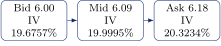
Figure 1. Bid, midpoint and ask translated into annual implied volatility for the same six-month call.
The local sensitivity of implied volatility to a price change is the reciprocal of vega:
\[d\sigma_{\rm imp}\simeq\frac{dC}{C_\sigma}.\]
The six-month call has vega 27.7895 per unit of volatility, so a one-cent price change implies about 0.036 volatility percentage points. With only two calendar days remaining, an otherwise comparable at-the-money call has vega about 2.9526; the same cent implies 0.339 points. At vega 0.25 it implies four points. A striking IV move in a very small premium can therefore arise from a single price tick. Reading it alongside the premium, spread and time to expiry gives a much clearer account of the observation.
A narrow, recent two-sided market anchors a fit more strongly than a wide or old quote when observations are weighted by their price uncertainty. Comparing fitted prices with the original bid and ask keeps the assessment in units a trader can act on.
3. Surfaces and price sensitivities
An option chain gives a set of implied volatilities at different strikes and expiries. A volatility surface connects them. To compare strikes across maturities we use the forward \(F_T=S e^{(r-q)T}\) and log-forward moneyness \(k=\log(K/F_T)\). Total variance is \(w(k,T)=\sigma(k,T)^2T\). For our call,
\[F_T=101.005017,\qquad k=-0.010000,\qquad w=0.020000.\]
These coordinates separate a strike’s position relative to the forward from the variance accumulated over the remaining life. For example, annual volatilities of 21%, 20% and 19% at three, six and twelve months correspond to total variances of 0.011025, 0.020000 and 0.036100. The downward-sloping volatility term structure still implies more accumulated variance at longer horizons.
The current Volt surface interpolates total variance linearly between log-moneyness points within an expiry and then between expiries. It answers queries within the supported strike and maturity range. This gives the application a transparent way to compare quotes and value intermediate contracts. Financial consistency adds another requirement. At a fixed expiry, call prices should decline with strike and form a convex curve. Put–call parity links calls and puts to the forward. The implementation checks these relations on its inspection grid, together with calendar total-variance consistency. Constrained surface models, including the arbitrage-free SVI construction of Gatheral and Jacquier [4], provide a stronger framework for controlling the shape throughout the fitted domain.
The second strike derivative of a smooth European call-price curve recovers a risk-neutral density,
\[f_Q(K)=e^{rT}\frac{\partial^2 C}{\partial K^2},\]
as shown by Breeden and Litzenberger [3]. A negative value points to inconsistent option prices or an unsuitable fit. A smooth-looking picture can therefore still require substantial correction before it supports valuation.
For a contract valued at a specified volatility, the familiar sensitivities are
\[\begin{align*} \Delta=C_S&=e^{-qT}N(d_1),\\ \Gamma=C_{SS}&=\frac{e^{-qT}\phi(d_1)}{S\sigma\sqrt T},\\ \nu=C_\sigma&=Se^{-qT}\phi(d_1)\sqrt T. \end{align*}\]
Here \(\phi\) is the standard normal density. Our call has delta 0.553457, gamma 0.0277895 and vega 27.789495. Delta measures the local value change for a dollar move in stock while holding volatility fixed. Gamma measures how that delta changes. A one-percentage-point volatility rise, from 20% to 21%, uses \(0.01\nu\), approximately 0.277895 per underlying unit.
Suppose the smile is held fixed in log-forward moneyness, with local volatility slope \(\sigma_k=-0.30\). When spot rises, our fixed-strike call moves along that smile. Since \(dk/dS=-1/S\), its volatility changes at \(\sigma_S=0.003\) per dollar, giving
\[\frac{dC}{dS}=C_S+C_\sigma\sigma_S=0.636826.\]
The difference from 0.553457 comes from the accompanying volatility movement. The application supports fixed-volatility partials and spot shocks that retain the fitted log-forward smile. An empirical model of smile dynamics would supply a further, data-dependent scenario rule.
If we change spot and re-solve volatility while requiring the call price to remain exactly 6.090127, the price stays at its target by construction. Differentiating that calibration gives \(C_S+C_\sigma\sigma_S=0\). For the example, the required volatility adjustment is about \(-0.019916\) per dollar. This calculation describes how the fitted parameter compensates for a changed input. For hedge risk, we instead specify the joint market movement we wish to evaluate and reprice along it. Automatic differentiation follows whichever dependencies we provide.
4. A stock hedge and the risks that remain
Now take ten short calls, each with multiplier 100. Signed contract quantities turn the per-unit calculations into portfolio amounts:
\[V=\sum_i n_i m_i C_i,\qquad G_V=\sum_i n_i m_i G_i.\]
Here \(n_i\) is signed contracts, \(m_i\) is the multiplier and \(G_i\) is a compatible per-unit sensitivity. The short calls have the following exposures at the unrounded theoretical mark.
| Quantity | Short-call position |
|---|---|
| Option value | \(-6{,}090.127\) |
| Delta, stock units | \(-553.457\) |
| Gamma, currency / squared price unit | \(-27.7895\) |
| Vega, currency per volatility point | \(-277.895\) |
| Theta, currency per calendar day | \(+17.7592\) |
| Rho, currency per rate basis point | \(-2.46278\) |
Theta measures calendar decay, using \(-C_T/365\) here. A rate basis point is 0.0001 in the annual rate. The option value belongs alongside the premium cash, stock position and financing account when calculating the complete book.
Buying 553.457 stock units offsets the initial delta. With whole shares, buying 553 leaves a small residual delta of approximately \(-0.457\). Even the exact fractional hedge retains curvature and volatility exposure, as the two instantaneous shocks in Figure 2 show.
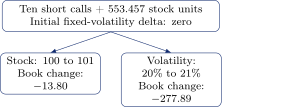
Figure 2. Full repricing of two separate shocks, with time and carry fixed. The stock shock holds volatility fixed; the volatility shock holds stock fixed.
For the stock move, the call reprices to 6.657382. The short calls lose 567.254 and the stock gains 553.457, giving a combined loss of 13.797. The local gamma estimate is \(\tfrac12\Gamma_V(\Delta S)^2=-13.895\), close to full repricing for this move. For the volatility shock, the call reprices to 6.368020 and the short calls lose 277.893. The stock value stays unchanged. A headline delta of zero therefore leaves economically significant exposures to monitor.
Under the log-forward smile rule above, stock 101 implies volatility \(0.20+0.30\log(101/100)=0.2029851\). The call then reprices to 6.740140. Comparing this result with the fixed-volatility result makes the consequence of the assumed smile movement concrete.
For a larger book, expiry and strike buckets locate the source of aggregate vega. Their calculation follows the surface mapping. If an option’s volatility is a linear blend of two bucket levels with weights 0.6 and 0.4, its bucket vegas are \(0.6\nu\) and \(0.4\nu\). Interpolation in total variance produces different weights through the chain rule. Full scenario repricing then checks the local approximation, especially for large moves, short expiries and concentrated positions. Realized trading results additionally include changes in holdings, execution prices, fees, dividends and funding.
5. Across stocks, sectors and factors
Six-month at-the-money volatility, a fixed-moneyness downside skew and the difference between short- and long-dated volatility each describe a specific part of a stock’s surface. Displaying their changes across a sector can reveal whether a repricing is broad or concentrated in one name. A useful exception might be an increase in one stock’s downside volatility while its peers remain stable. The next step is to inspect its quotes, upcoming events and liquidity, then compare the change with that stock’s own history. A wide spread can explain an apparent outlier before an economic explanation is needed.
Equity-factor exposures translate stock moves into a common portfolio scale. Let the simple stock return satisfy \(r_i=\sum_a B_{ia}f_a\), where \(f_a\) is a factor return and \(B_{ia}\) is the stock’s estimated loading. If \(\Delta_i\) includes both option and stock holdings, define cash delta \(D_i=S_i\Delta_i\). Then
\[\Delta V\simeq\sum_a E_a f_a,\qquad E_a=\sum_i D_i B_{ia}.\]
For cash deltas of \(+5{,}000\) and \(-3{,}000\), and loadings 1.2 and 0.8 to the same factor, \(E=3{,}600\). A 1% factor rise implies a first-order gain of 36. This comparison gives stock, sector and common-factor views of the same book. Shared currency units and the stated simple-return mapping make the aggregation interpretable; curvature and accompanying volatility movements enter fuller scenarios.
The equity loadings above map factor returns into stock-price changes. For vega exposure, we need loadings that map volatility-factor changes into movements of the option surface. Suppose \(\delta\sigma_i=\sum_b L_{ib}z_b\). With vega \(\nu_i\) measured per unit of annual volatility, the corresponding exposure is
\[H_b=\sum_i n_i m_i\nu_i L_{ib}.\]
The shocks \(z_b\) might represent a common volatility rise, a steeper downside smile or a change in the term structure. Estimating these movements requires a history of surfaces on comparable coordinates. It also allows a portfolio to carry little net equity-factor delta while retaining a large common volatility exposure.
Historical changes in surface levels, skews and term slopes can supply option-market factors. After scaling those changes consistently, principal components extract the combinations accounting for the most shared variation. An alternative first explains the changes with existing equity and sector factors, then studies the remaining common variation. This second route asks what information the option market adds to the return-factor model. Raw prices and their Greeks have strong mathematical relationships; choosing financially comparable features and evaluating them on later observations helps distinguish a useful new factor from a restatement of existing inputs.
A cross-sectional map shows comparable surface changes by stock and sector. An exposure view shows the signed book’s equity- and volatility-factor sensitivities. An exception list brings together unusual peer-relative changes and the quotes underlying them. Selecting a stock can connect all three views to its chain and to a repriced scenario. Price-change attribution adds another useful link:
\[\Delta C\simeq\Delta\,\Delta S+ \tfrac12\Gamma(\Delta S)^2+\nu\,\Delta\sigma+\Theta\,\Delta t.\]
For an interval with unchanged holdings, this explains the local stock, curvature, volatility and calendar contributions. Full repricing supplies the comparison; the remaining difference includes higher-order and interaction terms. Trade cash flows and changes in holdings complete an attribution of realized portfolio P&L.
The European quote API provides double-precision CPU inversion, fitted volatility and risk calculations for a single underlying [6]. Hypercube organizes the observations and calculated results [5].
6. An exercise-aware market viewer
Volt’s exercise-pricing worker supports American rights throughout a declared interval and Bermudan rights on explicit dates, including cash-dividend events. A producer submits dated quotes to POST /api/options-risk/frame; the panel receives completed results from GET /api/options-risk/snapshot. Implied volatility uses the stock observation paired with each option quote. Subsequent stock updates reprice the contract at that retained volatility until another option quote arrives. Saved snapshots also support file replay.
A historical capture supplies 64 American contracts across eight stock and ETF underlyings, arriving over about 24 seconds. Every contract received prices and Greeks. The replay supplies flat 4% continuously compounded interest, zero continuous yield and an empty cash-dividend schedule as modelling assumptions. Its illustrative book holds one long contract per row. Observed quotes and paired stock prices supply the market inputs.
The Options Risk panel groups signed exposures by underlying and lets the reader edit contract quantities. Wide spreads and quote ages accompany the calculated Greeks. Production use supplies the relevant carry and dividends.
References
[1] F. Black and M. Scholes. The pricing of options and corporate liabilities. Journal of Political Economy 81(3), 637–654, 1973. https://doi.org/10.1086/260062. Back to text ↑
[2] R. C. Merton. Theory of rational option pricing. Bell Journal of Economics and Management Science 4(1), 141–183, 1973. https://doi.org/10.2307/3003143. Back to text ↑
[3] D. T. Breeden and R. H. Litzenberger. Prices of state-contingent claims implicit in option prices. Journal of Business 51(4), 621–651, 1978. https://doi.org/10.1086/296025. Back to text ↑
[4] J. Gatheral and A. Jacquier. Arbitrage-free SVI volatility surfaces. Quantitative Finance 14(1), 59–71, 2014. Author preprint: https://arxiv.org/abs/1204.0646. Back to text ↑
[5] StrategyNet. Hypercube: architecture and publication interfaces, source documentation, October 2026. https://github.com/ingvor-restrat/hypercube. Back to text ↑
[6] StrategyNet. Volt: numerical companion and financial semantics, source documentation, October 2026. https://github.com/ingvor-restrat/volt. Back to text ↑
This walkthrough is for research and educational purposes. It illustrates how strategynet.ai organizes signal evidence into factors and scenarios. It provides no recommendation, investment advice, or instruction to trade any security.
Back to Insights