
Pricing and Hedging a Multi-Asset Option with Volt
October 2026 · research@strategynet.ai · Web edition
Original PDF · LaTeX source · Derivative portfolio risk
An option linked to several stocks can become most exposed to whichever stock leads the group. A hedge must respond as that exposure moves between names, and early exercise can bring the contract to an end before expiry. Valuing the remaining rights and financing the hedge therefore require a joint model of the underlying prices and a consistent account of exercise and trading. We develop this application in Volt using a Bermudan call on the largest of five stock prices. Neural continuation functions determine the holder’s exercise decisions; independent simulations then estimate its payment value and a policy-tail upper valuation. The selected holder can also supply settlements to a writer that learns vector hedge holdings through the native application interface. A declared reconstruction of a published pricing experiment provides the numerical comparison. Three independently initialized models recover prices between 26.1576 and 26.1609 against the published 26.154, with wider confidence intervals. The application exposes the market model, backward learning calculation, valuation estimator and financed account through runnable interfaces, with independent numerical controls for CPU, Metal and CUDA execution.
1. The contract and market model
Consider a holder who receives the amount by which the best-performing stock exceeds a strike. With \(d\) underlying prices \(S^1,\ldots,S^d\) and strike \(K\), the cash payment on exercise is
\[g(S_t)=\left(\max_{1\leq i\leq d} S_t^i-K\right)^+.\]
A different stock can lead at each date. That changes the distribution of future payments and the stock positions useful to the writer. The Bermudan contract adds a decision for the holder: exercise now or retain the remaining opportunities. Our application follows this decision through valuation and then into the writer’s trading account.
The comparison uses Becker, Cheridito and Jentzen’s five-asset case [1]. All stocks start at 100, strike is 100, maturity is three years, and nine equal exercise intervals give a four-month calendar. Each stock has annual volatility 20% and continuous dividend yield 10%; the interest rate is 5%. Under the pricing law \(\mathbb Q\),
\[dS_t^i=(r-q_i)S_t^i\,dt+\sigma_i S_t^i\,dW_t^i.\]
Thus the ex-dividend drift in this case is \(-5\%\). The published row uses independent Brownian components. The same generator accepts a supplied correlation matrix and heterogeneous stock parameters.
For a time increment \(\Delta t\), the exact GBM transition is
\[S_{t+\Delta t}^i=S_t^i\exp\!\left[ (r-q_i-\tfrac12\sigma_i^2)\Delta t+ \sigma_i\sqrt{\Delta t}\,Z_i\right].\]
The vector \(Z\) is standard Gaussian with the specified correlation. A semidefinite Cholesky factor permits perfectly correlated assets as well as full-rank inputs. Checked reconstruction and roundoff diagnostics accompany the factorization. Indexed random streams bind every stock path to its seed, namespace, global path ID and dates, so streaming batches retain their identities.
A portfolio application supplies different liabilities through the same financial interface. The max-call is useful here because the published benchmark supplies a concrete pricing target, while the underlying joint process and vector account exercise the multi-asset implementation.
2. Backward continuation learning
Write \(G_n=e^{-rt_n}g(S_{t_n})\) for a payment discounted to time zero. Suppose a later exercise rule \(\tau_{n+1}\) has already been chosen. The continuation function at date \(n\) estimates
\[c_n(x)=\mathbb E^{\mathbb Q}[G_{\tau_{n+1}}\mid S_{t_n}=x].\]
The regression network minimizes squared error against the future rule’s realized discounted payments. Once fitted, it exercises where \(G_n\geq c_n(S_{t_n})\). Moving backward from expiry supplies the later rule needed to fit each earlier date. All decisions use the observed state when applied to a new path.
The state contains the five raw stock prices and the current discounted unit payoff. Two hidden tanh layers each have 55 units; a linear output gives the continuation value in currency per option unit. Batch normalization acts on the input and hidden affine outputs. The final fitted date receives Xavier initialization. Each earlier date starts from the next date’s weights and normalization statistics, with fresh Adam moments.
The article reports a declared reconstruction of the published settings. The paper specifies the architecture, batch size, total update counts and learning-rate values. We record the remaining choices explicitly: normalization placement and population moments, epsilon 0.001, running-statistic weight 0.01 for new observations, Xavier-uniform kernels, finite path reuse, and Adam’s bias-corrected denominator with epsilon \(10^{-8}\).
The final date uses 6,000 updates, with rates 0.1, 0.01, 0.001 and 0.0001 for 1,000, 2,000, 2,000 and 1,000 updates. Earlier dates use 3,500 updates with 500, 1,000, 1,500 and 500 updates at those rates. Batch size is 8,192. Each model uses 1,048,576 training paths and 65,536 separate diagnostic validation paths. Row sampling is uniform with replacement from resident training tensors.
The scheduled final snapshot at every date supplies the primary exercise rule and earlier training targets. Separate validation snapshots remain diagnostic. This fixes selection before fresh pricing paths are generated. Completed-date archives retain the market identities and selected future networks, allowing an interrupted fit to restart the next earlier date reproducibly.
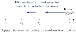
Figure 1. Training proceeds backward. Pricing and trading follow new paths forward, preserving the information available at each decision.
3. Independent policy-tail valuation
A selected holder produces an expected discounted payment \(L=\mathbb E^{\mathbb Q}G_{\tau}\). Its admissible stopping rule makes \(L\) a lower value relative to optimal exercise. A sample mean estimates \(L\) with Monte Carlo uncertainty. An upper expectation can be constructed from the policy’s value martingale using nested conditional simulation [2], [1].
At each outer state \(X_n\), simulate independent future paths that continue past the current date and apply the selected holder from \(n+1\). Their average payment \(\overline C_n\) estimates the continuation of that actual future rule. If \(f_n\) is the binary exercise decision on the outer state, define
\[\Delta\widetilde M_n=f_nG_n+(1-f_n)\overline C_n-\overline C_{n-1}, \qquad \overline C_N=0.\]
Starting from \(\widetilde M_0=0\), accumulate these increments from date one. Each conditional mean is reused in its two adjacent increments. The upper estimate averages \(\max_n(G_n-\widetilde M_n)\) along the full outer path, including exercise opportunities after the holder’s first stopping date.
This noisy process is the policy-value martingale plus conditionally centered simulation error relative to the outer observations. The paper’s conditional Jensen argument supplies the upper expectation. The conditional simulations retain their own random addresses for each parent state, date and child; each outer observation also has its own initial continuation estimate. Pooling several parent groups into a device batch preserves those addresses and each parent’s payoff summation.
The assessment uses 4,096,000 lower-estimate paths, 2,048 upper outer paths and 2,048 conditional branches per state. Three selected models share common assessment market streams, allowing their realized payments to be compared. Training, validation, outer and conditional sampling have separate declared random domains. Reported intervals use the outer-sample standard errors and an asymptotic joint 95% lower/upper enclosure. The lognormal max-call is unbounded, so this calculation uses its finite-variance sampling assumptions.
For the chosen source row, the published lower and upper estimates are 26.156 and 26.152, with midpoint 26.154 and enclosure \([26.138,26.171]\). Finite sample estimates can cross even though their population expectations obey the lower/upper inequalities. Our reports retain their observed ordering. Before fitting, we set two numerical comparison targets: absolute midpoint difference at most 0.05 and enclosure width at most 0.10. Both proximity and precision enter the assessment.
4. The writer’s vector account and application API
The selected holder can supply settlements to a writer. For continuous yield \(q_i\), use discounted dividend-reinvested security values
\[P_n^i=e^{(q_i-r)t_n}S_{t_n}^i.\]
These share the time-zero currency basis of \(G_n\). Cash growth is one, and a holding \(h_n^i\) corresponds to \(h_n^i e^{q_i t_n}\) physical shares. Reinvestment is included in the security definition.
Let \(w_n\) be wealth before rebalancing and let \(\lambda_i\) be proportional stock costs. Choosing target holdings \(h_n\) gives arrival wealth
\[w_{n+1}^{-}=w_n- \sum_i\lambda_iP_n^i|h_n^i-h_{n-1}^i| +\sum_i h_n^i(P_{n+1}^i-P_n^i).\]
At exercise, the account liquidates its hedge, charges the declared closing cost and pays the signed discounted liability once. Later holdings remain zero. Quantity and multiplier scale the payment once; the caller supplies initial capital for the complete position.
The native writer observes current stocks, discounted unit payoff and previous holdings, then chooses a vector of continuous targets. Its complete-account squared-loss objective differentiates through trades, fees and settlement. The supplied writer example uses date-specific ReLU networks and this terminal account objective. The paper’s interval hedge method instead learns changes in approximate continuation value using reinvested-stock features.
maxcall_episodes verifies the actual holder checkpoint’s digest, applies its first admissible exercise decision and prepares native scenario batches. The existing training, evaluation, holdings-inference and checkpoint operations accept those batches. Jormungandr can supervise the same Volt worker through its native HTTP service [3].
cargo build --release -p volt-compute --bin maxcall_learning --bin maxcall_episodes --bin native_learner
python3 examples/maxcall_application.py --output /tmp/volt-maxcall-example
The example fits a holder, prepares independent writer training/validation ranges, selects a writer checkpoint and assesses its restored version on fresh paths. Inputs, costs, normalization, market identities and model snapshots accompany the outputs. A small default run demonstrates the full sequence, while the published-case study uses the larger declared budgets. The background primer develops the contract and account arithmetic [4].
5. Precision and device performance
The primary price comparison uses CPU float64. Independent calculations check normalization, all parameter gradients, optimizer moments and post-update inference.
Single-precision tests identified a sensitive normalization representation. A constant hidden affine bias is removed by the following batch normalization, and an input-normalization translation is likewise removed by the next normalized affine layer. In exact arithmetic these are redundant training directions. Small floating-point cancellation residuals can be amplified by Adam, while stored running means adjust over time.
Volt exposes an optional fixed-zero representation for these translations. Converting an existing network also adjusts the following running means, so its represented inference function is preserved. The remaining biases and normalization shifts retain their learned roles. Independent Keras and NumPy controls check both the converted and already-fixed forms on CPU, Metal and CUDA. The original raw comparison and the stabilized comparison remain separate in the evidence records.
The performance workload uses the same network, inputs, normalization, arithmetic and precision across its compared devices. Each block restores common weights and statistics. Warm-up updates precede synchronized measured updates; simulation, upload, first-use setup and readback retain separate measurements. CPU runtimes use one thread. Device memory requirements are checked before allocation and recorded alongside actual runtime telemetry. The implementation builds on Burn’s tensor/autodiff interfaces and CubeCL execution, using the repository’s pinned versions [5].
6. Pricing results and execution times
All three independently initialized models passed the comparison targets. Their midpoint estimates were 26.1576, 26.1609 and 26.1589, respectively, against the published 26.154. The absolute differences ranged from 0.0036 to 0.0069, and each joint enclosure had width about 0.0745. The source row’s published enclosure has width 0.033; the present estimates therefore achieve close price agreement with wider sampling uncertainty.
| Model | Lower | Upper | Midpoint |
|---|---|---|---|
| Published | 26.1560 | 26.1520 | 26.1540 |
| Volt A | 26.1393 | 26.1759 | 26.1576 |
| Volt B | 26.1427 | 26.1790 | 26.1609 |
| Volt C | 26.1407 | 26.1771 | 26.1589 |
The respective joint 95% enclosures were \([26.1206,26.1950]\), \([26.1239,26.1984]\) and \([26.1221,26.1964]\). Common assessment paths couple the three results; the three initializations measure training variability under that shared assessment. Every checkpoint was selected and archived before the first assessment result was opened.
Each full CPU float64 fit completed 30,500 updates in about 770 seconds. The three fits ran concurrently, with one CPU thread per fit. This duration includes the complete backward training sequence and its progress checks; independent pricing follows as a separate calculation. The terminal-only European value is 23.0516, obtained by independent integration of the maximum-price distribution. Early exercise adds about 3.11 in this case.
A separate CUDA fit uses float32 with fixed translations. Its 30,500-update fit took 263 seconds, followed by 66 seconds for full fresh-path valuation. Its midpoint was 26.1592 with joint enclosure \([26.1220,26.1969]\). Common-path payments from this policy and the unchanged CPU reference were statistically compatible. Complete-fit durations combine hardware, precision and representation choices; the matched table below compares the same declared arithmetic workload.
The optional fixed-translation representation passed twelve independent controls spanning CPU float64/float32, Metal float32 and CUDA float32, with both converted and already-fixed initial states. The original float32 representation exposed post-update discrepancies in the redundant translations; those observations motivated the explicit alternative.
The matched float32 measurements below use the optional fixed-translation representation and strict native-dtype products. All eighteen CPU/GPU workload comparisons passed the numerical controls. Each entry is the median of sixty measured updates across three restored blocks, each preceded by three warm-ups. Update times include forward/backward calculation, Adam, synchronization and scalar checks. Here ms means milliseconds.
| Apple M3 Max | Linux workstation | ||||
| \(d\) | Batch | CPU | Metal | CPU | CUDA |
| 5 | 256 | 0.65 | 7.08 | 1.39 | 5.38 |
| 5 | 1,024 | 2.33 | 9.67 | 4.34 | 3.05 |
| 5 | 8,192 | 16.62 | 38.02 | 38.48 | 11.91 |
| 10 | 256 | 0.73 | 6.79 | 1.50 | 2.89 |
| 10 | 1,024 | 2.44 | 8.79 | 5.45 | 3.14 |
| 10 | 8,192 | 18.57 | 41.94 | 41.97 | 11.19 |
| 50 | 256 | 1.34 | 8.66 | 2.38 | 2.76 |
| 50 | 1,024 | 4.54 | 10.29 | 9.48 | 3.56 |
| 50 | 8,192 | 34.89 | 56.68 | 77.69 | 16.13 |
The Mac runs macOS 27.0.1 with 128 GiB unified memory. The Linux system uses one CPU thread on a Threadripper PRO 7985WX and an RTX 4090 with 24 GiB device memory, CUDA 12.5 and driver 555.42.02. Both use Rust 1.99.1 and Burn 0.22.1. Metal fusion is enabled; CUDA uses the qualified unfused configuration. Background host utilization was recorded throughout, including concurrent CPU training on the Mac. These are measurements under that observed load.
CPU execution was faster than Metal throughout these training cases. CUDA became useful at batch 1,024: the five-stock case reached a 1.42-fold update speed ratio over its same-host CPU, increasing to 3.23-fold at batch 8,192. The fifty-stock, batch-8,192 ratio was 4.81. A larger state and resident batch provide enough arithmetic to amortize device dispatch and synchronization.
First-use work also matters. For five stocks and batch 8,192, the first training update took about 629 ms on Metal and 2,039 ms on CUDA. First inference and readback took 103 and 412 ms respectively, while warmed inference/readback took 1.62 and 0.63 ms. These first-touch figures include the existing compiler/cache state. The full timing record separates parameter setup, upload, first use and steady updates, making it possible to choose a device for the actual request.
Independent tests cover market moments, financed cash flows, conditional sampling, completed-date recovery and executable checkpoint provenance.
This study establishes one five-asset pricing comparison and a runnable vector hedging application. Other contract parameters and hedge objectives can be assessed through the same interfaces. Factor forecasts and live vendor inputs require their own calibration and observation-timing studies.
References
[1] S. Becker, P. Cheridito and A. Jentzen. Pricing and hedging American-style options with deep learning. JRFM 13(7):158, 2020. https://arxiv.org/abs/1912.11060v3. Back to text ↑
[2] S. Becker, P. Cheridito and A. Jentzen. Deep Optimal Stopping. JMLR 20(74):1–25, 2019. https://jmlr.org/papers/v20/18-232.html. Back to text ↑
[3] Volt. Multi-asset market, learning and complete writer application guides. https://github.com/ingvor-restrat/volt/blob/main/docs/multi-asset-maxcall.md. https://github.com/ingvor-restrat/volt/blob/main/docs/maxcall-learning.md. https://github.com/ingvor-restrat/volt/blob/main/docs/maxcall-application.md. Back to text ↑
[4] StrategyNet. Options, Exercise and Learned Hedging: A Practical Primer. 2026. https://github.com/ingvor-restrat/volt/blob/main/docs/latex/compute/volt_option_learning_primer.pdf. Back to text ↑
[5] Burn project. Tensor, automatic-differentiation and execution architecture. https://burn.dev/books/burn/. Back to text ↑
This walkthrough is for research and educational purposes. It illustrates how strategynet.ai organizes signal evidence into factors and scenarios. It provides no recommendation, investment advice, or instruction to trade any security.
Back to Insights