
Learning to Hedge with Stocks and Options: The Control Problem, Learning Method and Application Interfaces
October 2026 · research@strategynet.ai · Web edition
Original PDF · LaTeX source · Derivative portfolio risk
A dealer who sells an option must finance its eventual payment while managing the risk of market moves along the way. Trading stock offsets some of that exposure; adding a traded option gives the dealer another way to manage curvature and volatility risk. Every adjustment also incurs costs. We formulate this decision as a finite-horizon stochastic control problem, specifying the market dynamics, observations, holdings, cash account and terminal loss. We explain how squared loss and conditional value at risk lead to different learning objectives, and how a neural policy learns from complete trading paths through automatic differentiation. Volt supplies the financial calculation and learner, while Jormungandr supplies the training and inference interfaces. A worked cash account, a dated decision timeline and a tail-loss diagram connect the mathematics to an application. Numerical comparisons and a synthetic learning exercise demonstrate the calculation and its application interface. The client workflow covers scenario submission, training, held-out evaluation, holdings inference and checkpoint recovery.
1. Hedging an option book
A dealer sells a call on a stock and receives its premium. At expiry, the buyer can claim the excess of the stock price over the agreed strike. A put pays the excess of the strike over the stock price. Selling both at the same strike creates a short straddle: the dealer owes a payment when the stock finishes far enough in either direction. The premium finances the hedge, but the eventual payment and the trading needed to manage it remain uncertain.
A stock position offsets the option book’s response to a small price change. Delta measures that response, in shares per option unit. Gamma measures how delta changes as the stock moves. Vega measures the response to a change in volatility, with its quoted unit specified by the application. These exposures change during the life of the book. A trader who continually adjusts a stock hedge therefore pays transaction costs while retaining exposure to movements between trading times and to changes in option prices.
A second option adds another way to manage that risk. Let \(L\) denote the liability and \(C\) a traded call used for hedging. Given their model Greeks, a delta–gamma hedge holds
\[\begin{equation} h^C=\frac{\Gamma_L}{\Gamma_C},\qquad h^S=\Delta_L-h^C\Delta_C. \end{equation}\]
The call offsets curvature and the stock completes the delta adjustment. The remaining vega is \(\nu_L-h^C\nu_C\); its size depends on the chosen contracts. A small hedge-option gamma can also produce a very large call position. Instrument choice, position limits and trading costs matter as much as the local sensitivity calculation.
Deep hedging learns the holdings from simulated trading experience [1]. François and colleagues develop the stock-and-option setting using joint index returns and implied-volatility information [2], [3]. The policy receives current observations and existing positions, then selects the next stock and option quantities. Training rewards decisions that reduce a specified measure of the final hedging loss after costs and financing. This is useful when a simple Greek-matching rule trades too frequently, or when several instruments offer different combinations of risk reduction and execution cost. Model hedges still provide valuable comparisons: they explain what the neural policy gains or gives up as the market and cost assumptions change.
2. The market and the decision process
Write the trading dates as \(t_k=k\Delta t\), \(k=0,\ldots,N\). The episode ends at \(T=t_N\). The policy chooses holdings at \(k=0,\ldots,N-1\); the final date settles the liability and sells the hedge. Daily trading means one action per trading day. Simulation may use finer time steps to construct prices between those dates while preserving the chosen trading frequency.
Figure 1 follows one trading episode. Each decision uses the observations and holdings available at that date; the final loss supplies the training signal for all preceding actions.
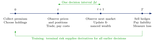
Figure 1. One episode follows the liability from sale to expiry. The policy acts at specified dates using information available at that date. Prices move between decisions; financing and trading costs enter the account before the terminal objective is calculated. Training repeats this calculation across many market paths.
A market generator describes how the external market state \(X_k\) changes:
\[\begin{equation} X_{k+1}=F_k(X_k,\varepsilon_{k+1}),\qquad \varepsilon_{k+1}\sim P_k(\,\cdot\mid X_k). \end{equation}\]
The scenario probability law determines which outcomes the objective weights. A risk-neutral law supports a pricing-model benchmark; an estimated real-world law supports a hedge assessed under that return distribution. Both require consistent instrument marks and financing assumptions. Here \(X\) can contain the stock price, volatility variables, interest rates and any additional factors required by the model. The current examples treat the trader as a price taker: changing the hedge affects wealth and costs, while the external price process follows its own law. Market impact would require a transition model with the action among its inputs.
The two-day application control uses geometric Brownian motion,
\[\begin{equation} S_{k+1}=S_k\exp\!\left[(r-q-\tfrac12\sigma^2)\Delta t +\sigma\sqrt{\Delta t}\,\varepsilon_{k+1}\right], \end{equation}\]
with independent standard-normal innovations, \(\Delta t=1/252\), \(S_0=100\), \(\sigma=0.20\), \(r=0.03\) and \(q=0.01\). The liability pays \(|S_2-100|\). The hedge call has strike 100 and an initial 84-trading-day maturity; its mark at each date is its Black–Scholes value using the remaining maturity and those same parameters. These choices completely specify this small market experiment.
The separate Heston study lets instantaneous variance \(v\) change randomly:
\[\begin{align} dS_t&=\mu S_t\,dt+S_t\sqrt{v_t}\,dB_t,\\ dv_t&=\kappa(\bar v-v_t)\,dt+\xi\sqrt{v_t}\,dW_t,\\ d\langle B,W\rangle_t&=\rho\,dt. \end{align}\]
Mean reversion has speed \(\kappa\) and long-run variance \(\bar v\); \(\xi\) controls fluctuations in variance and \(\rho\) connects the two shocks. Our zero-rate Heston comparison uses \(\mu=0\), \(S_0=100\), \(v_0=\bar v=0.04\), \(\kappa=1\), \(\xi=2\), \(\rho=-0.7\) and 30 daily intervals of \(1/365\). Its second hedge instrument is a funded variance claim. That experiment and the two-day stock-and-call control have different market and instrument definitions. Each has its own scenario and result records.
The full economic state is \((k,X_k,V_k,h_{k-1},u_k)\): date, market variables, account wealth, existing holdings and any running contract statistic \(u_k\). An Asian payoff, for example, requires a running average. The agent receives an observation vector \(x_k=\phi_k(X_{0:k},u_k)\) and its previous holdings. The application chooses which quantities to expose. If a latent volatility factor is omitted, the observed problem can require memory to infer it. Wealth can also be supplied as a feature when the policy should react to it. The supplied two-day policy observes scaled log spot and time remaining, plus previous holdings.
The action \(h_k=(h_k^S,h_k^C)\in\mathbb R^2\) specifies the desired stock and option holdings. Orders are the changes \(h_k-h_{k-1}\). The current continuous-output native policy permits signed quantities; adding position limits requires a specified admissible action set and its implementation. The initial holdings are zero and initial wealth is the premium. The account recurrence below, together with \(F_k\) and the terminal payoff, defines the controlled system completely.
3. Stock, option and cash positions
The account starts with wealth \(V_0\), typically the premium collected for the liability. At each trading time \(t\), the policy chooses stock shares \(h_t^S\) and hedge-option units \(h_t^C\). Let \(H_t=(S_t,C_t)\) be their prices, and let \(h_{-1}=0\). With proportional trading fees \(\kappa_i\), the cash left after rebalancing is
\[\begin{equation} c_t=V_t-h_t^S S_t-h_t^C C_t -\sum_{i\in\{S,C\}}\kappa_i H_t^i|h_t^i-h_{t-1}^i|. \end{equation}\]
This cash balance earns or pays interest. Under a stock dividend-reinvestment convention, the next pre-trade wealth is
\[\begin{equation} V_{t+1}=c_t R_t+h_t^S S_{t+1}G_t+h_t^C C_{t+1}, \end{equation}\]
where \(R_t=\exp(r_t\Delta t)\) and \(G_t=\exp(q_t\Delta t)\). The scenario input supplies these growth factors, allowing the account convention to be checked alongside the prices. A negative cash balance represents borrowing.
At the liability’s expiry, the remaining hedge positions are sold. With closing-cost rates \(\kappa_i^{\rm close}\), the available wealth and loss are
\[\begin{align} V_T^{\rm liq}&=V_T-\sum_i\kappa_i^{\rm close}H_T^i|h_{T-1}^i|,\\ E_T&=L_T-V_T^{\rm liq}. \end{align}\]
A positive \(E_T\) is a shortfall; the seller’s profit is \(-E_T\). The longer-dated hedge option is sold at its expiry-date market value while the liability pays its contractual amount. Each opening, adjustment and closing fee enters the account once.
Consider a one-period example. A dealer sells one call with strike 95 for a premium of 6. The stock costs 100 and a longer-dated hedge call costs 4. Buying 0.4 shares and 0.5 hedge-option units costs 42. Stock fees of 5 basis points and option fees of 1% add 0.04, leaving cash of \(-36.04\). Over the period, that borrowing grows by a factor of 1.001. The stock then reaches 102 and the hedge call 4.8; dividends are zero.
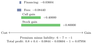
Figure 2. Sources of profit in the two-date example. Bar lengths show currency contributions from trading gains, fees and financing. The premium and liability add a net cost of one currency unit.
The profit can also be reconstructed from stock gains of 0.8, option gains of 0.4, the original premium of 6, the liability payment of 7, total fees of 0.0844 and financing of 0.03604. Both calculations give 0.07956. This independent reconstruction helps catch sign and timing errors.
Contract multipliers must be applied consistently. An exchange contract covering 100 shares corresponds to 100 option units when option prices are quoted per share. The stock quantity is already in shares. The application converts contracts to these economic quantities once, before constructing the account. The same convention carries through premiums, Greeks, fees and terminal payments. Scaling the entire example by 100 scales every cash flow and the profit by 100; mean squared loss then scales by \(100^2\).
4. Learning from completed trading paths
The policy is a function \(h_t=\pi_\theta(x_t,h_{t-1})\), where \(x_t\) contains information available at the trading time and \(\theta\) contains learned weights. Spot, time to expiry, option quotes and volatility descriptors can all be inputs. Existing holdings tell the policy how much its next decision will cost to implement. Features drawn from a full future path must be restricted to observations available at \(t\).
For \(B\) scenario paths, one objective is mean squared hedging loss,
\[\begin{equation} J(\theta)=\frac1B\sum_{b=1}^B E_T^{(b)}(\theta)^2. \end{equation}\]
This penalizes both overfunding and shortfall. Downside squared loss replaces \(E_T^2\) by \(\max(E_T,0)^2\), emphasizing the seller’s unpaid obligation. Conditional value at risk, or CVaR, concentrates on the worst losses. Its level-\(\alpha\) representation is
\[\begin{equation} \operatorname{CVaR}_\alpha(E_T)=\min_\eta \left\{\eta+\frac{\mathbb{E}[(E_T-\eta)_+]}{1-\alpha}\right\}. \end{equation}\]
In reinforcement-learning notation, intermediate rewards can be set to zero and the final reward to \(-\ell(E_T)\), with discount factor one. For squared loss, \(\ell(e)=e^2\). For CVaR at a given threshold \(\eta\),
\[\begin{equation} \ell_\eta(e)=\eta+\frac{(e-\eta)_+}{1-\alpha}. \end{equation}\]
Optimizing \(\eta\) alongside the policy yields the CVaR objective; the native empirical calculation evaluates the equivalent fractional-tail statistic. Funding already appears in the cash account. The trader commits at the start to the chosen terminal-risk objective and learns a policy for that objective across the full horizon. This formulation gives each action credit through its eventual effect on the account, including future trading costs.
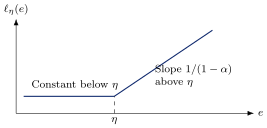
Figure 3. CVaR training puts additional weight on losses above the threshold. Increasing \(\alpha\) concentrates the objective on a smaller, more adverse part of the loss distribution.
The native learner supports squared, downside squared, empirical CVaR and entropic objectives. Its empirical CVaR calculation weights a fractional observation at the tail cutoff when the requested tail size is nonintegral. Choice of objective changes the trading problem: a policy trained on average squared error can differ materially from one protecting against extreme shortfall.
The terminal liability and trading account determine the training signal. The learner runs each path forward, calculates the final loss, and propagates derivatives back through all holdings, fees and cash balances to the weights. An optimizer then changes those weights. Every decision date receives its learning signal from the final loss. Known model hedges provide independent performance comparisons. The supplied continuous-action application uses this direct differentiation approach within Jormungandr’s learner interface.
Burn carries out automatic differentiation through the tensor calculation [9]. For exogenous simulated prices, those prices are fixed inputs during a weight update; derivatives follow the policy and the account. Absolute-value trading costs are piecewise differentiable, with the implementation’s derivative convention at zero turnover. Price Greeks use differentiation with respect to financial inputs; policy training uses differentiation with respect to network weights. Volt provides both applications, with distinct inputs and outputs.
For a batch of trajectories \(\omega_b\), the actual update is
\[\begin{equation} \widehat J(\theta)=\frac1B\sum_b\ell(E_T(\theta;\omega_b)),\qquad \theta\leftarrow\operatorname{Adam}(\theta,\nabla_\theta\widehat J). \end{equation}\]
The implemented method is direct policy optimization through a differentiable simulator/account calculation. It uses the known derivatives of that calculation to learn continuous actions. Other RL methods can estimate a value function or a policy gradient from sampled rewards; integrating one of those engines would retain the same economic problem specification. A policy’s output is the next holding, and its training target is the risk of the resulting account.
The current native policy uses a separate two-hidden-layer ReLU network at each decision date and feeds previous holdings into the next decision. It learns for the liability and scenario distribution supplied during training. At deployment, changing market observations changes the action through \(x_t\). Supporting a broader range of books requires liability descriptors and representative portfolios in the training distribution, followed by validation across those books. Equivalent contractual decompositions should produce the same net cash flows and economic exposures under matched costs; that property can be tested directly in the account and policy inputs.
5. Training and inference through the API
A hedging application supplies its scenarios and liability, then uses the same model for training, evaluation and holdings inference. Volt evaluates the financed account and differentiates its chosen risk objective. Jormungandr manages the model and exposes the requests over HTTP [4], [5]. A registered worker retains the policy, optimizer and scenario tensors between requests. CPU, Metal and CUDA builds select where that calculation runs.
The following Python calls use JormungandrClient. Start the service with VOLT_LEARNER_BIN pointing to the compiled Volt worker. The public example examples/native_hedging.py launches two scenario-producing actors against it [5]. Here we follow one model through the same API, using the two-day market defined in Section 2.
Here premium is the initial straddle value under the stated pricing model. The default policy has two decision dates, two market features, two hedge instruments and hidden width eight. Setting the objective to {"kind":"cvar","alpha":0.95} selects 95% CVaR; changing the risk preference leaves the scenario submission workflow intact.
A batch supplies flattened arrays: marks has shape \([B,N+1,2]\), features has \([B,N,2]\) and payoffs has \([B]\). For each path the marks alternate stock and call prices at successive dates. Features contain scaled log spot and time remaining at each decision. The array payoffs holds the straddle payment owed at expiry. Each batch also carries its path count and dataset identity with its first path index. Registering disjoint ranges assigns the observations to training and validation before the tensors are uploaded.
Training consumes the uploaded training batch and advances the model version once per accepted update. Evaluation measures the current policy on the separate validation batch. Replacing or streaming training batches extends this loop to larger scenario sets. Multiple actors can submit work to one model using the same versioned update protocol. The supplied example implements retries after an actor receives a stale-version response.
For a current market observation, inference returns target stock and option holdings. With spot 100, normalized log spot zero and the full two-day horizon remaining, the input uses features \([0,1]\) and zero previous holdings.
The returned holdings vector uses the stock and call ordering of the scenario marks. The application subtracts its current holdings to form orders. A checkpoint preserves model weights, Adam moments, configuration and dataset declarations. Restoring it reproduces holdings inference; continued training re-uploads the required scenario tensors. The client releases resources with client.delete_native_model(model).
These calls map directly to HTTP: model creation uses POST /v2/native/models; the other operations use POST /v2/native/models/{id}/{operation}. Applications can use these routes from another language or register another compatible policy engine. The worker keeps the financial tensors and optimizer in its execution backend; the application receives holdings, risk summaries and versioned model state.
The request sequence below creates the learner, submits two scenario batches, trains it, evaluates held-out paths, retrieves holdings and restores a checkpoint. The premium and scenario batches are the inputs described above.
import math
from jormungandr.client import JormungandrClient
client = JormungandrClient("http://127.0.0.1:8080")
model = "hedge"
client.create_native_model({
  "model_id": model, "backend": "volt_burn",
  "config": {
    "target": "cpu", "precision": "f64",
    "premium": premium,
    "objective": {"kind": "squared_loss"},
    "trading_costs": [0.0005, 0.01],
    "liquidation_costs": [0.0005, 0.01],
    "cash_growth": [math.exp(0.03/252)] * 2,
    "income_growth": [math.exp(0.01/252), 1.] * 2}})
client.native_command(model, "register_dataset", {
  "dataset_id": "gbm-study", "partitions": [
    {"split": "train", "first_path": 0, "paths": 64},
    {"split": "validation", "first_path": 64,
     "paths": 64}]})
for name, batch in [("train", training_batch),
                    ("validation", validation_batch)]:
    client.native_command(model, "upload", {
      "batch_id": name, "split": name, "batch": batch})
for _ in range(30):
    version = client.get_native_model(model)["version"]
    client.native_command(model, "update", {
      "batch_id": "train", "expected_version": version})
report = client.native_command(model, "evaluate", {
  "batch_id": "validation"})
targets = client.native_command(model, "infer", {
  "step": 0, "paths": 1, "features": [0., 1.],
  "previous_holdings": [0., 0.]})
state = client.native_command(model, "checkpoint")
state.pop("ok", None)
client.create_native_model({"model_id": "resumed",
  "backend": "volt_burn", "checkpoint": state})
6. Validation and measured results
We checked the trading calculation against a second implementation that follows each market path one date at a time using ordinary numbers and loops. It pays for holdings and fees, accrues interest and settles the liability. Both versions were written for this project; their separate code paths help catch sign errors, missing charges and incorrect payment timing. Parameter derivatives were also checked by perturbing weights and comparing the resulting change in loss.
The CPU double-precision checks agree to roughly \(10^{-15}\) across the loss, parameter derivatives and first optimizer update. The corresponding CPU/Metal single-precision checks agree to roughly \(10^{-6}\) for path profits. The validation records retain the individual errors and test inputs.
A companion comparison also executed the original Deep Hedging author’s published financial engine and network components [6]. With matched inputs, both implementations reached validation CVaR of approximately 0.262 in a two-date Black–Scholes learning control after 1,000 updates.
The matched Heston application extends this check to 30 hedge dates, stock and a funded variance instrument. Three paired training seeds used the same initial weights, 131,072 training paths, 8,192 validation paths and 10,000 updates. On 32,768 fresh common paths, mean policy CVaR was 0.28700 for the author implementation and 0.28896 for Volt. The author-minus-Volt interval was \([-0.00828,0.00463]\) at the adjusted 95% level. The model hedge produced 0.24552. Increasing both the training and validation pools substantially improved both learning engines relative to their earlier small-pool fits.
The learner also provides volt_shared_lstm_reset: two shared long short-term memory (LSTM) layers followed by two dense ReLU layers and linear holdings outputs. Its hidden state resets at each decision, following the reference implementation’s one-observation sequence. Optional wealth inputs carry the financed account into the decision and remain connected through differentiation during training. Dropout has an explicit probability and seed. CPU and Metal/fusion checks cover forward holdings, financial loss, all parameter derivatives, the first Adam update and checkpoint continuation.
The two-date API example uses a constant-volatility stock process, a straddle liability and stock plus a longer-dated call as hedge instruments. Two actors submit batches and update one model. The example checks the complete client workflow on a small calculation; the larger study below evaluates hedging performance on a joint return and implied-volatility model.
Executing the stock-and-option author’s complete agent class checks the new engine directly. With shared inputs and weights, holdings, financed profits and the first optimizer update agree to approximately \(10^{-6}\) in single precision. The reference profile uses the author’s recurrent activation, learned small-trade threshold and Adam epsilon convention.
The reference-rule study trained three shared policies for 1,000 updates each, with batches of 1,000 paths. Training used 32,000 paths, validation used 4,000 separate paths, and assessment then used 8,000 fresh common paths. Its liability was one quoted-unit 63-day at-the-money straddle; hedges were stock and an 84-day at-the-money call. Stock trades cost 0.05% and option trades 2%. At maturity, the stock position is valued at its mark and call liquidation incurs the 2% fee. The generator used the coefficients supplied by the reference example. Validation used the smooth trading rule; final inference used the specified sharpening operation. The selected updates were 1,000, 1,000 and 900.
Mean squared hedging loss averaged 0.344, compared with 3.756 for the source delta control, 2.408 for delta–gamma hedging using pricing Greeks, and 30.581 without hedging. Mean fees were 0.624 for the learned policies and 1.150 for delta–gamma hedging. The learned-minus-delta–gamma MSE difference was \(-2.063\), with an adjusted 95% interval of \([-2.450,-1.880]\). One path in 8,000 crossed the declared intermediate tracking limit for each policy. All policy selections were fixed before generating the assessment paths.
A further comparison uses a classical trading band. Validation selected a threshold of three for the sum of absolute changes in stock and call holdings. On 4,000 additional fresh common paths, learned MSE was 0.286, band MSE 1.333, and daily delta–gamma MSE 2.250. Mean fees were 0.625, 0.711 and 1.150, respectively. The adjusted learned-minus-band MSE interval was \([-1.118,-0.974]\). The same three neural checkpoints were retained, and the band threshold was selected before generating these paths. This comparison shows an advantage beyond the cost savings of the selected fixed band.
These results describe the supplied simulator and finite training budget. The original paper’s historical calibration, path filtering and longer training experiment provide further comparisons. An earlier 200-update sigmoid-LSTM variant is retained in the research record; its separate 8,000-path assessment produced mean squared loss of 0.462.
| CPU workload | Volt | PyTorch |
|---|---|---|
| 64 paths, 2 dates, width 8 | 0.355 | 0.360 |
| 256 paths, 30 dates, width 17 | 5.957 | 5.440 |
Table 1. Median warm training-update time in milliseconds on an Apple M3 Max, macOS, float64, one CPU thread per runtime. Each update includes the trading calculation, backward differentiation and Adam optimization.
The timing comparison used five warm-up updates and 20 alternating measured updates. Volt used a tuned release build with ThinLTO and native CPU targeting. Its time includes worker communication; PyTorch runs in process. Initial upload and model creation are excluded. These measured workloads are small; the table provides an execution reference for the application calculation.
Application checks also cover dataset-partition enforcement, stale model versions, checkpoint continuation and a different registered learner engine.
7. Using the workflow in a trading application
The same interfaces support a research comparison and a deployed decision process. For research, the application uploads common held-out market paths and evaluates the learned policy alongside delta and delta–gamma hedges, using the same premiums, instrument units, financing and execution costs. Loss, turnover and account paths then explain the economic effect of the policy. The mathematical market specification stays with the dataset so that the comparison can be reconstructed.
For ongoing decisions, the application prepares the observation using the training-time feature definitions, supplies current holdings and requests the next target. The step index selects the policy for the remaining horizon. Stock and option prices, contract maturity and any volatility features must use the same conventions as training. Portfolio quantities convert the targets into economic exposures; the execution application handles order sizes, liquidity and position controls.
8. Exercise decisions and the writer’s hedge
A put holder can receive \(\max(K-S_t,0)\) by exercising. American rights permit this throughout the contract’s life; Bermudan rights specify a finite set of dates. Exercising gives up the remaining option, so the holder compares that payment with the expected value of waiting. The writer’s hedge runs until the resulting stopping time \(\tau\), when the claim settles.
Let \(G_n=e^{-rt_n}\max(K-S_{t_n},0)\) denote a discounted put payment under the risk-neutral model. A continuation function estimates the expected discounted payment from a later exercise rule:
\[c_n(x)=\mathbb{E}^{\mathbb Q}[G_{\tau_{n+1}}\mid S_{t_n}=x].\]
Backward regression fits this expectation by squared error, then exercises where \(G_n\geq c_n(S_{t_n})\). The 2019 direct method instead learns a smooth exercise probability \(f_\theta(x)\) by maximizing
\[\mathbb{E}^{\mathbb Q}\!\left[G_n f_\theta(S_{t_n})+ (1-f_\theta(S_{t_n}))G_{\tau_{n+1}}\right].\]
Later decisions stay fixed while fitting the current date. Deployment uses the resulting binary exercise decisions. Volt implements both methods from Becker, Cheridito and Jentzen [7], [8], starting with a one-stock GBM put and an explicitly dated exercise grid.
The holder and writer optimize different quantities. The holder seeks the largest expected discounted payment under the pricing model. Given that rule, the writer chooses hedge holdings to reduce its selected after-cost risk. Volt’s finite-difference holder map supplies an independently computed exercise control, including cash dividends. Its scenario producer supplies either numerical or learned stopping times to the writer’s native worker. An upload adds exercise with per-path settlement indices and signed amounts, cash_income for intermediate per-unit payments, and optional initial_wealth for per-path starting capital. The existing native_command upload, update and evaluation calls remain the application interface.
At settlement the account liquidates the hedge, pays the liability and finances cash to the common final date. This makes the reported loss comparable across early and late exercise paths. Separate checks reconcile the payments, dividend credits, fees and parameter gradients, and the HTTP test reproduces the next optimizer update after checkpoint restoration.
For frictionless interval hedging, the 2020 method fits stock holdings against changes in approximate option value. Write \(P_n=e^{(q-r)t_n}S_{t_n}\) for discounted, dividend-reinvested stock and \(v_{n+1}=\max(G_{n+1},c_{n+1})\) at the next exercise opportunity. The regression minimizes
\[\mathbb{E}^{\mathbb Q}\!\left[ \bigl(c_n+h_n(S_{t_n})(P_{n+1}-P_n)-v_{n+1}\bigr)^2 \right].\]
Volt exposes this interval calculation separately from the complete-path after-cost writer objective. Fresh-path valuation reports the learned holder’s payment estimate and a nested conditional-value martingale upper estimate, with sampling uncertainty. The implemented martingale uses a continuation proxy; the papers also describe policy-tail constructions. The numerical pricing model, exercise dates and financial assumptions remain part of each comparison.
Our complete-account exercise study sells one put on one share, with spot and strike 100, one-year maturity, 20% constant volatility and 5% funding. The stock follows risk-neutral GBM. The holder uses the numerical rule on four quarterly exercise dates; the writer can hedge monthly. Three seeds per cost setting each trained for 3,000 updates on 16,384 paths, with 4,096 validation paths. Each date has a width-16, two-hidden-layer network, using log stock price, remaining time and previous holdings. All six selections preceded generation of 16,384 fresh common assessment paths.
| Stock fee | Learned | Numerical delta | Trading band |
|---|---|---|---|
| 0 | 4.013 | 3.935 | 3.937 |
| 10 basis points | 4.079 | 3.984 | 3.986 |
Table 2. Fresh-path mean squared terminal-bank loss for the Bermudan writer. Learned entries average three selected policies. The stock-holdings band was selected on validation.
Leaving the liability unhedged gives mean squared loss of 61.443. The learned hedge therefore removes roughly 93% of that squared loss and finishes about 2% above numerical delta at this training budget. Adjusted 95% paired intervals for the learned-minus-delta difference are \([0.045,0.110]\) without fees and \([0.050,0.141]\) with fees. Replaying all 98,304 learned-policy paths through a separate cash calculation agrees within \(10^{-12}\). This study evaluates the writer against the numerical holder; learned-holder valuation and interval hedging have their own objectives and assessment paths.
A separate holder study permits exercise at all twelve monthly dates. Each algorithm uses three seeds, 32,768 training paths, 8,192 validation paths and 500 updates per fitted date. After selecting all six holders and three interval hedges, assessment uses 65,536 paths for holder payments and 4,096 outer paths with 64 conditional children for the martingale estimate. Across the six holders, payment estimates range from 5.952 to 5.983 and upper estimates from 6.262 to 6.292. Every asymptotic 95% price enclosure contains the matching finite-difference value of 6.0428; doubling its mesh from 600 to 1,200 changes the value by about 0.00013. The roughly 0.3 estimator gap leaves scope for more accurate continuation fits and additional conditional simulation.
On 32,768 additional paths, the three interval hedges have discounted-error MSEs of 3.986–4.116, compared with 54.57–58.60 for cash alone at their declared training-derived initial capital. These studies establish the one-stock application and its checks. The papers’ multidimensional max-call experiments, larger training schedules and published numerical tables provide the next replication comparison.
Changing the liability or market model begins with a new scenario specification. Longer horizons, additional instruments and new market observations enter through the configured policy dimensions and batch arrays. Predictive factors can enter as features when their observation times and training distribution are defined. This gives practitioners a common way to study whether additional information or a different hedge instrument improves risk after trading costs.
References
[1] H. Buehler, L. Gonon, J. Teichmann and B. Wood. Deep Hedging. 2018. https://arxiv.org/abs/1802.03042. Back to text ↑
[2] P. François, G. Gauthier, F. Godin and C. O. Pérez-Mendoza. Deep Hedging with Options Using the Implied Volatility Surface. 2025, arXiv:2504.06208v3. https://arxiv.org/abs/2504.06208v3. Back to text ↑
[3] C. O. Pérez-Mendoza. Author reference implementation and experiment configuration. https://github.com/cpmendoza/deep-hedging_with_options. Back to text ↑
[4] Volt. Native learner application guide. Protocol, financial inputs, execution backends and checkpoint support. https://github.com/ingvor-restrat/volt/blob/main/crates/volt-compute/docs-native-learner.md. Back to text ↑
[5] Jormungandr. Native learners. Application endpoints, registered engines and example client. https://github.com/ingvor-restrat/jormungandr/blob/main/docs/native-learners.md. Back to text ↑
[7] S. Becker, P. Cheridito and A. Jentzen. Deep Optimal Stopping. JMLR 20(74):1–25, 2019. https://jmlr.org/papers/v20/18-232.html. Back to text ↑
[8] S. Becker, P. Cheridito and A. Jentzen. Pricing and hedging American-style options with deep learning. JRFM 13(7):158, 2020. https://arxiv.org/abs/1912.11060. Back to text ↑
[9] Burn. Tensor and automatic-differentiation implementation. https://github.com/tracel-ai/burn. Back to text ↑
This walkthrough is for research and educational purposes. It illustrates how strategynet.ai organizes signal evidence into factors and scenarios. It provides no recommendation, investment advice, or instruction to trade any security.
Back to Insights