
Learning to Hedge in Volt: Models, Decisions and Evidence
October 2026 · research@strategynet.ai · Web edition
Original PDF · LaTeX source · Derivative portfolio risk
Investors use options to protect portfolios against losses and to take positions on future market movements. An option gives its buyer the right to buy or sell an asset at an agreed price and under specified exercise terms. The institution selling the contract takes on the corresponding obligation, whose value can change substantially before settlement. Hedging is the practice of holding other positions to offset changes in that obligation. As prices and volatility move, those positions need adjustment. Frequent rebalancing incurs trading costs, while delaying a trade leaves the institution exposed to further market moves. The practical problem is to decide when to trade, which instruments to use and how much risk to retain after paying for the hedge. Deep Hedging approaches this problem by learning trading decisions from simulated market paths. The policy is trained to reduce a specified measure of terminal loss after transaction costs, allowing the cost of a trade to be weighed against its effect on subsequent risk. Volt provides the market-path calculations, financed trading account, risk objectives and policy optimization for these studies. Jormungandr exposes a persistent learner through training, evaluation, holdings-inference and checkpoint APIs. We study European option liabilities under Heston stochastic volatility using stock and a funded variance claim as hedge instruments. The completed 21-case comparison shows how learned policies adapt to trading costs, including improvements over model-Greek hedges executed at the same dates and fees. A separate conditioning study removes 87% of the observed gap to the model hedge by changing the scales used in training. Worked examples and application calls show how practitioners can construct the same kind of experiment, compare hedges on common scenarios and retrieve decisions from a trained policy.
1. The cost of maintaining an option hedge
Consider a dealer who sells a call option. A rise in the stock price increases the value of the claim owed to the buyer. Buying stock offsets some of that increase. In the Black–Scholes model, the dealer can replicate the claim by holding its delta in stock and continuously adjusting that position, provided trading is frictionless and the model assumptions hold.
In practice, the dealer trades at discrete times and pays a spread or fee on each adjustment. Following every small change in model delta can consume the premium through trading costs. Waiting saves costs but leaves the book exposed to the next price move. Stochastic volatility adds another source of risk, which calls for an additional hedge instrument. Options or variance instruments can help, but their cost and sensitivity introduce further choices. The relevant question is how to manage the whole book over its remaining life within a specified tolerance for loss.
Deep Hedging [1] learns a policy for these repeated decisions. At each date, a network uses the observed market state and current holdings to select the next position. Training evaluates the resulting terminal profit after costs across simulated paths. A tail-loss objective can favour protection against adverse outcomes; increasing trading costs can favour retaining an existing position through small market moves. The objective expresses the dealer’s preference, while the simulator supplies the market conditions under which that preference is optimized.
Our Heston experiment hedges a European call with stock and a funded variance claim. We compare terminal losses and trading costs with model hedges and with the numerical results reported in the original Deep Hedging study.
2. Financing, loss preferences and required capital
Start with a dealer who has sold a call paying \(Z=\max(S_T-K,0)\). At time zero the dealer receives premium \(p\) and buys \(\delta_0\) shares. With zero interest, the cash balance becomes \(p-\delta_0S_0\). Selling those shares at maturity and paying the claim gives
\[P_T=p-Z+\delta_0(S_T-S_0).\]
The cash account funds the initial purchase, and the gain identity includes that financing explicitly.
As an illustrative arithmetic example, take \(S_0=K=100\), \(p=5\), and \(\delta_0=0.5\). If \(S_T=110\), profit is \(5-10+5=0\) and the unhedged claim loses 5. If \(S_T=90\), the same hedge earns \(5-0-5=0\) and the unhedged claim earns 5. These chosen endpoints illustrate the offsetting exposure. At the intermediate price \(S_T=100\), the half-share hedge leaves profit of 5.
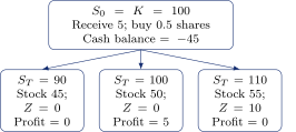
Figure 1. Stock and cash match the claim at 90 and 110. The middle outcome retains profit of 5. Stock entries give terminal values; each profit includes the cash balance.
The same cash accounting extends to a sequence of trades. Write \(M_k\) for the instrument marks at date \(k\) and \(\delta_k\) for the holdings chosen there. The purchases and sales then telescope into
\[\begin{split} P_T={}&p-Z+\sum_{k=0}^{n-1}\delta_k\cdot(M_{k+1}-M_k)\\ &-\sum_{k=0}^{n}c_k(\delta_k-\delta_{k-1}). \end{split}\]
Here \(\delta_{-1}=0\) and final inventory is liquidated. The last cost is included according to the declared terminal-cost convention. A proportional cost is \(\varepsilon M_k|\delta_k-\delta_{k-1}|\) for a positive-priced hedge asset. Funding, dividends and borrow costs need their own cashflows when nonzero.
The training graph evaluates this identity in floating point. A second route records purchases, cash, fees, settlement and liquidation using Volt’s exact financial units. Agreement catches errors such as charging a fee twice, misplacing a multiplier or using tomorrow’s price for today’s trade. Converting research holdings to fixed-point quantities introduces a separate quantization error, which is bounded and reported. Exact ledger balance proves the accounting identity. Hedge quality and simulator accuracy have separate empirical tests.
CVaR ranks policies by their losses in the worst part of the distribution. Write terminal profit as \(P\) and loss as \(L=-P\). Upper-tail CVaR at confidence \(\alpha\) is
\[R_\alpha(P)=\min_\eta\left[ \eta+\frac{\mathbb{E}[(L-\eta)^+]}{1-\alpha}\right].\]
The threshold \(\eta\) is optimized alongside the policy. At \(\alpha=0.99\), the criterion concentrates on the worst one percent of losses; it needs enough independent tail observations to be estimated reliably.
Consider five equally likely, invented terminal outcomes:
| Policy | 1 | 2 | 3 | 4 | 5 |
|---|---|---|---|---|---|
| A profit | \(-8\) | \(-2\) | 1 | 2 | 3 |
| B profit | \(-3\) | \(-1\) | 0 | 0 | 0 |
Both mean profits are \(-0.8\). Their 0.8-CVaRs are 8 and 3: the worst fifth contains one outcome. Their 0.5-CVaRs are 3.8 and 1.6, using fractional mass at the loss threshold of the worst 2.5 observations. The example shows why the risk preference changes the preferred decision while expected profit stays fixed. The inputs are chosen for this worked example.
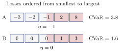
Figure 2. At \(\alpha=0.5\), the shaded tail contains two full observations and half an observation at the median threshold \(\eta\). Each full box represents probability 0.2.
A dealer who wants to penalize increasingly large losses smoothly can use entropic risk:
\[R_\lambda(P)=\lambda^{-1}\log\mathbb{E}[e^{-\lambda P}].\]
This criterion penalizes losses exponentially; \(\lambda\) has reciprocal currency units. For small fluctuations it behaves approximately as \(-\mathbb{E}[P]+\lambda\operatorname{Var}(P)/2\). Squared loss \(\mathbb{E}[P^2]\) instead penalizes deviations on both sides of zero. Each objective has its own interpretation and numerical scale.
CVaR and entropic risk translate a cash premium into an equal reduction in risk. This cash-invariance property is \(R(P+p)=R(P)-p\). Let \(G_\delta\) be the after-cost trading gain. The associated indifference capital is
\[p^*=\inf_\delta R(G_\delta-Z) -\inf_\delta R(G_\delta).\]
The second optimization asks what trading alone can achieve in the same market. Its subtraction separates the liability capital from a potentially profitable trading opportunity. A report using comparison premium \(q\) therefore contributes \(q+R(q+G_\delta-Z)\) before subtracting the optimized empty-liability risk. Squared loss changes quadratically when the cash premium changes and therefore requires its own capital convention.
3. The Heston market, hedge instruments and simulation
Heston models the stock price and its instantaneous variance jointly. In our zero-rate benchmark they follow
\[dS_t=S_t\sqrt{V_t}\,dB_t,\qquad dV_t=\kappa(\theta-V_t)dt+\xi\sqrt{V_t}\,dW_t,\]
where \(B\) and \(W\) are correlated Brownian motions. \(S\) is the underlying asset price; \(V\) is its instantaneous variance, whose drift reverts toward \(\theta\). Negative correlation lets falling prices coincide with rising variance. The stock drift is zero in this benchmark. Its stochastic law determines the conditional scenarios used for training and evaluation.
The control problem has a 30-date horizon. At each date the policy observes its configured stock/variance features and previous holdings, then chooses signed target quantities in stock and the variance claim. Trading changes the financed account through gains and proportional costs; the market evolves under the stochastic equations above. The episode ends with the European liability payment. Training minimizes the specified terminal-risk objective using derivatives through the complete trading path. The stock-and-option application article develops the state, observation, action and reward formulation explicitly, with a complete training and inference workflow through Jormungandr.
The target starts at \(S_0=100\), \(V_0=\theta=0.04\), with \(\kappa=1\), \(\xi=2\), correlation \(-0.7\) and 30 daily decisions of length \(1/365\). The large volatility of variance makes excursions toward zero important. These parameters lie below the Feller positivity condition \(2\kappa\theta\geq\xi^2\), so the simulation must handle that region carefully. Clipping negative Euler draws would change the transition law.
The two independent diffusion risks motivate a second benchmark instrument, a funded integrated-variance claim. If \(A_t=\int_0^tV_s\,ds\) and \(\tau=T-t\), its conditional mark is
\[H_t=A_t+a(\tau)(V_t-\theta)+\theta\tau, \quad a(\tau)=\frac{1-e^{-\kappa\tau}}{\kappa}.\]
For a smooth option mark \(C(t,S,V)\), a local model hedge uses
\[\delta^S=C_S,\qquad \delta^H=\frac{C_V}{a(\tau)}.\]
This matches the variance diffusion as well as the stock diffusion before maturity, where \(a(\tau)>0\). Large numerical holdings in \(H\) partly reflect its small per-unit variance scale. Each instrument needs its own price, risk units and notional convention for economic comparison. As maturity approaches, \(a(\tau)\) shrinks, so division by it can amplify numerical errors in \(C_V\).
The model hedge uses the known Heston parameters and is rebalanced at the same 30 decision dates as the learned policy. This finite trading grid leaves replication error. The minimum attainable CVaR can lie below the model hedge’s risk, and trading costs create another opportunity to improve the objective. A policy can accept a different tail-loss distribution or save the cost of small trades. A learned policy that trails this feasible reference retains a measurable performance gap even after improving on the unhedged book.
We sample variance exactly at each date from the CIR conditional distribution, using a Poisson–gamma mixture. To generate the stock between dates, we approximate the variance accumulated over that interval with left or trapezoid quadrature. The time step therefore affects the resulting stock paths. The formal study uses the uncorrected trapezoid construction; Broadie and Kaya describe the full exact joint procedure [3], [4].
In an earlier million-path common-input control, left integration produced a call value of 1.703843 (standard error 0.002189), whereas trapezoid produced 1.693466 (0.002164); the independent continuous-Heston price was 1.691834. More paths narrow sampling uncertainty; step refinement addresses discretization bias.
The completed saved-strategy resolution study keeps 30 decisions and 31 marks while using 30, 60 or 120 simulation steps. Its 600 evaluations cover all selected policies and their empty-liability controls on 65,536 diagnostic paths per resolution; 4,800 ledger audits pass. The one-system mean squared hedging loss is 0.304750, 0.303037 and 0.303849; the five-system MSE is 1.801082, 1.791411 and 1.787311. These observed shifts are small relative to the model-hedge gaps reported below.
The 600 evaluations reuse the selected learned strategies. The paired control reported below also revalues the model and band hedges on common paths within each resolution. Both studies retain the same 30 decision dates. Each resolution has its own simulated paths, so the comparison intervals describe strategy differences within that resolution.
4. Learning the trading policy
At date \(k\), the policy observes stock price, variance and current inventory, then computes its next holdings:
\[\delta_k=F_k(\log S_k,V_k,\delta_{k-1};w_k).\]
The date-specific networks use two hidden ReLU layers and signed linear outputs. Inventory is useful information: the cost of buying another share depends on what is already held. The Markov ablation removes inventory from the policy inputs. It restricts the policy information while retaining the same ledger and fee schedule.
Each simulated path produces a liability payment, hedge gains and trading costs. Training differentiates the batch risk measure through those cashflows to update the network weights. The model hedge supplies a separate performance comparison; its holdings are used as training labels only in the supervised diagnostic reported later.
A call spread from strikes 100 to 110 pays the same amount as the sum of spreads 100–105 and 105–110 at the same expiry. Both constructions pay 7 when the terminal stock price is 107, and agree at every other terminal price. If their cashflow timing, funding and trading constraints agree, the same hedge policy has the same P&L under either construction. The payoff engine aggregates the contracts before the network evaluates their trading consequences. Our call-plus-put versus straddle regression checks this property for values, risk objectives and parameter gradients.
Two books can have the same local exposures but different losses after a large move or a change in volatility. Different exercise rights, collateral or cashflow dates can also change the trading problem despite similar terminal payoff diagrams. A policy trained for one liability should therefore be reused for an alternative construction when its payoff, timing, funding and trading economics agree. Training across genuinely different books would require portfolio information as an input and examples covering those changes during training.
For one simulated trajectory, the training computation follows
\[\begin{gathered} \text{state}\longrightarrow\delta_0\longrightarrow \text{next state and inventory}\\ \longrightarrow\delta_1\longrightarrow\cdots \longrightarrow P_T\longrightarrow R. \end{gathered}\]
When inventory enters the next decision, differentiating through the whole sequence includes its effect on later actions. Detaching previous actions would remove part of that gradient. Market draws are exogenous here: policy weights affect holdings and costs while the sampled market trajectory stays fixed. Modelling price impact would extend the transition model so that trades also affect subsequent market states.
CVaR introduces a hinge at the loss threshold. Proportional costs introduce an absolute value at zero trade. Valid subgradient conventions permit training, and the resulting neural optimization remains nonsmooth and nonconvex. Validation selects among the parameter states reached by this search; establishing global optimality would require additional analysis.
Suppose the current stock holding is 0.50 and the new local target is 0.51. At stock price 100 and proportional cost \(1/512\), changing by 0.01 costs about 0.001953 per option unit. A trade earns its place when the expected reduction in risk exceeds that cost. Small changes can therefore create an inaction region around the current holding.
A transparent control projects the current holding onto a band around the model target: retain inventory inside the band and trade to the nearest edge outside it. A separate validation cohort selects the band widths, which are then held fixed for final evaluation. This reference tests the value of the neural policy’s additional complexity.
Variance is around 0.04 in this experiment, while the funded variance hedge can require hundreds or thousands of instrument units. Rescaling the input and output units can improve conditioning while preserving the represented function class. These unit choices also affect initialization and the optimizer’s trajectory, so we track conditioned runs separately from the initially unscaled parameterization. Batch normalization adds another state: its saved inference statistics must represent the training distribution. Our training-stream recalibration controls exposed an early case that trained successfully but failed after saving.
For deployment, we save the weights and normalization statistics together. Validation and subsequent use apply those parameters to each new market observation.
5. Using Volt and Jormungandr
Volt provides the scenario-based financial calculation, policy optimization, held-out evaluation and saved policies used in this workflow. Applications can also control a persistent Volt learner through Jormungandr’s native API. The caller supplies the liability premium, market observations, instrument marks and execution assumptions. Volt follows the resulting trading account and returns the selected risk measure and policy holdings [15], [16].
The client creates a model from a configuration, registers disjoint dataset ranges and uploads training and validation batches. Once those inputs are registered, the training and decision calls are:
version = client.get_native_model(model)["version"]
client.native_command(model, "update", {
  "batch_id": "train", "expected_version": version})
result = client.native_command(model, "evaluate", {
  "batch_id": "validation"})
target = client.native_command(model, "infer", {
  "step": step, "paths": 1, "features": observation,
  "previous_holdings": current_holdings})
state = client.native_command(model, "checkpoint")
Here client is a JormungandrClient connected to the service, model identifies the configured learner, and the observation follows its training-time feature definitions. The returned target uses the same instrument order and units as the scenario marks. The application forms trades by subtracting its current holdings. Model configuration selects the risk objective; supported choices include squared loss, downside squared loss, CVaR and entropic risk.
The persistent API supplies date-specific continuous-output networks with inventory feedback and retained optimizer state. The experiment records specify the architecture used for each reported study. CPU/GPU selection, scenario-batch streaming and model checkpoints share the same application interface. The public guides provide the complete schemas and executable examples [15], [16].

Figure 3. Training learns decisions through their financial consequences. Independent ledger checks validate the accounting along the forward route.
6. Empirical results
6.1. Completed held-out comparison
| Completed held-out case | Learned risk | Model risk | Difference | 95% interval for difference |
|---|---|---|---|---|
| BS, entropic, cost \(1/64\) | 1.771132 | 4.162756 | \(-2.391625\) | [\(-2.399336\),\(-2.384290\)] |
| Heston, entropic, cost \(1/64\) | 1.497589 | 4.903836 | \(-3.406246\) | [\(-3.447575\),\(-3.375949\)] |
| Heston, 0.5-CVaR, recurrent | 0.369091 | 0.241897 | 0.127194 | [0.125583,0.128787] |
| Heston, 0.5-CVaR, Markov | 0.265136 | 0.241897 | 0.023239 | [0.019194,0.027473] |
| Heston, one system, MSE | 0.302964 | 0.144959 | 0.158005 | [0.154977,0.160901] |
| Heston, five systems, MSE | 1.805284 | 0.719825 | 1.085460 | [1.054311,1.134692] |
The table summarizes the completed formal study. We calculate each selected policy’s risk on the common one-million-path held-out cohort and report the average over five independent training fits. All methods within a case use the same marks, payoff, premium, hedge dates and fee convention. Lower risk is better; the difference is learned minus model. Entropic, CVaR and squared-loss rows measure different preferences on their respective numerical scales.
Intervals use 1,999 full-cohort hierarchical bootstrap replicates, resampling paths and the five fitted policies while preserving strategy pairing. The predeclared two-target adjustment is retained for the primary 0.5-CVaR and one/five-system cases; the other displayed intervals are pointwise 95%. Their coverage is conditional on the selected policies and simulator, with the stated family adjustment. Historical-source and simulator uncertainty require additional evidence.
At cost \(1/64\), the learned policies achieve lower after-cost entropic risk in both markets. The model hedge follows diffusion sensitivities and pays for every resulting trade; the learned policy can leave small exposures unadjusted. A stronger comparison uses a model hedge with a no-trade band selected on separate validation paths. Its risk is 1.891032 in BS and 2.562694 in Heston for these rows, so the learned policies also improve on that declared band control. At smaller BS costs some selected bands perform better, and the zero-cost Heston gaps remain.
The recurrent 0.5-CVaR capital estimate is 2.060925 with interval [2.058880,2.062886], compared with the original paper’s printed 1.94. The Markov case yields capital of 1.956970 [1.952751,1.961525]. It changes the policy specification and remains above the printed target. Its training streams and initialization also differ; a causal recurrence comparison requires those inputs to be controlled. The one/five-system learned MSEs also exceed the original 0.20 and 1.13 targets.
6.2. Implementation and historical checks
The author’s later sample engine outputs a trade \(a_k\), while Volt’s policy returns target holdings \(\delta_k\). They are related by \(a_k=\delta_k-\delta_{k-1}\). With zero initial inventory and the declared terminal-cost convention, the gain expressions satisfy
\[\sum_{k=0}^{n-1}a_k\cdot(M_n-M_k) =\sum_{k=0}^{n-1}\delta_k\cdot(M_{k+1}-M_k).\]
The comparison converts holdings into trades before evaluating gains and fees, using the same payoff sign and loss convention in both implementations.
We compared Volt with the author’s published financial engine, risk objective and neural network [10], using identical test cases and an explicit conversion from holdings to trades. The checked cash flows, holdings and parameter derivatives agree within \(10^{-6}\) in the single-precision comparison. A trained Volt policy also reproduces its path profits through the author’s network and financial engine.
These comparisons use the author’s later sample engine. Its world defaults and policy choices evolved after the original Heston experiments. The matched test supplies common external paths and aligned network inputs. Historical experiment comparisons additionally carry the market generator, architecture, normalization, optimizer, initial conditions and training budget.
A separate two-date control feeds prior holdings into the next network. It checks both the resulting holdings and the derivatives through that feedback. Detaching earlier holdings changes the gradient, as expected when earlier decisions affect the cost of later trades.
A matched two-date Black–Scholes control completed 1,000 updates using 512 training paths and 2,048 validation paths. Validation CVaR finished at 0.26150 for the author implementation and 0.26156 for Volt, compared with 0.44826 unhedged and 0.26872 for the same-fee delta hedge.
Rounding the CVaR tail to a whole observation changes the estimator whenever the selected tail contains fractional probability mass. For five losses \(4,1,0,-1,-2\) and confidence 0.7, the worst 1.5 observations have mean \((4+0.5\times1)/1.5=3\). Averaging the worst two instead gives 2.5. The comparison records each estimator and its convention explicitly. The original million-path tail counts at the specified confidence levels are integers.
The 21-case comparison contains five independent training fits per case: 105 liability fits and 95 separately optimized empty-liability fits. All 200 fits completed, and the saved models were checked for consistent training configuration and evaluation state. Selected weights were held fixed before the final cohort was used. The completed comparisons cover risk, capital, validation-selected bands and historical targets, retaining every declared configuration and fit.
Across the 23 declared historical targets, seven are compatible with our estimates, 13 are discrepant and three remain unresolved. These labels compare the printed rounded values with uncertainty under our simulator. The original study’s sampling and optimization uncertainty is unavailable, and some figures leave the loss statistic undefined. The 0.5-CVaR capital and the one/five-system scaling targets show clear discrepancies. Taken together, the results leave historical recovery incomplete.
A separate paired-resolution comparison evaluates learned, model and band hedges on 32,768 fresh paths at each of three simulation resolutions, retaining 30 hedge decisions. The conditioned zero-cost policy’s CVaR gap to the model hedge is 0.01951, 0.01844 and 0.01794 at one, two and four substeps. For the entropic-risk case with proportional cost \(1/256\), the learned-minus-band differences are \(-0.13788\), \(-0.13560\) and \(-0.13833\). The corresponding 95% intervals use 1,999 paired bootstrap replicates with adjustment for 18 comparisons, and retain these signs. Finer simulation preserves both the remaining zero-cost gap and the cost-case advantage. Comparisons pair strategies on common paths within each resolution; the three resolutions use separate path cohorts.
A conditioned, width-17 Markov network was trained to reproduce model holdings, using 4,096 complete training paths and 1,024 validation paths. Three fits of 10,000 updates are then assessed on 1,024 independent test paths. Their 0.5-CVaRs are 0.250283, 0.249667 and 0.258849, compared with 0.234125 for the adaptive model teacher and 1.454551 unhedged; all 32 ledger audits pass. The resulting holding errors measure approximation of a specified hedge; risk-objective training also has to discover useful holdings from terminal profit. Late variance-claim holdings retain sizeable fitting errors: the final-date RMSE is 1,233–1,263 instrument units. Evidence here covers those three Markov fits and their test cohort. Recurrent policies and broader state coverage extend the approximation question.
The completed conditioning comparison uses four network parameterizations, three independent fits per parameterization and 100,000 updates per fit. Training and validation data are matched across the four configurations; 131,072 common, independent confirmation paths evaluate the selected policies. The table averages the three policy CVaRs for each configuration. The model hedge’s 0.5-CVaR is 0.239966 on this cohort.
| Configuration | CVaR | Gap to model |
|---|---|---|
| Original units, recurrent | 0.389215 | 0.149250 |
| Scaled trades and feedback | 0.263288 | 0.023323 |
| Plus scaled state inputs | 0.258981 | 0.019015 |
| Conditioned Markov | 0.260293 | 0.020327 |
Scaling trade outputs and inventory feedback changes CVaR by \(-0.125927\), with interval [\(-0.131150\),\(-0.120778\)]. Adding state-input scaling gives a further change of \(-0.004308\) [\(-0.007424\),\(-0.001402\)]. The fully conditioned recurrent setup therefore removes 87.3% of the unscaled recurrent setup’s observed gap to the model. Its remaining difference is 0.019015 [0.016115,0.021810]. Comparing the two conditioned configurations gives a risk difference of 0.001312 [\(-0.001376\),0.004239], measured as Markov minus recurrent.
These 95% intervals use 1,999 paired bootstrap replicates, with a Bonferroni adjustment for seven declared comparisons. They resample both the three fits and the common paths. The result supports the complete training parameterization: changing the scales also changes the initial physical holdings, and the Markov configuration changes the input information. This development comparison uses fresh data and retains the completed historical assessment described above.
The remaining 0.019015 CVaR difference is about 7.9% of the model hedge’s 0.239966 CVaR on this confirmation cohort. Its practical size also depends on the liability premium, portfolio notional, available capital and the tail-loss preference. Statistical significance here describes sampling and training variation under the declared experiment. The causal explanation remains open. Scaling alone removed 87.3% of the earlier observed gap, showing how strongly the numerical setup can affect learning.
The completed comparisons also identify the settings that must travel with a reproducible experiment: initial physical holdings, input/output scales, batch normalization, network memory, Adam epsilon convention, training schedule and market discretization. The recorded author-code controls compare common paths and weights, derivatives, parameter updates and a learning run. CPU/GPU precision and reduction order belong in that sequence because small numerical changes can alter a long nonlinear optimization trajectory [14]. Matched forward and gradient controls already show close agreement in the cases tested. The recorded result therefore characterizes the declared training setup.
6.3. Matched Heston training with the author’s implementation
The larger matched experiment used 30 hedge dates, stock and a funded integrated-variance instrument, with two width-17 hidden layers. Three paired seeds shared paths and initial weights. Each engine completed 10,000 updates using 131,072 training paths and 8,192 validation paths, followed by assessment on 32,768 fresh common paths.
Mean policy CVaR was 0.28700 for the author implementation and 0.28896 for Volt, compared with 0.24552 for the model hedge and 1.44924 without hedging. The author-minus-Volt difference was \(-0.00196\), with an adjusted 95% interval of \([-0.00828,0.00463]\). The learning implementations agree closely under this specification, while the model hedge retains lower measured tail risk.
Earlier policies trained on 8,192 paths and selected on 4,096 paths produced CVaRs of 0.46150 and 0.45563 on the same fresh cohort. Increasing both pools reduced CVaR by roughly 0.17 in each engine. The comparison preserved initial weights, nested scenario prefixes, objectives and update counts. It shows how strongly sample settings affect this application and establishes a foundation for the next studies. Exact recovery of the original historical tables remains an additional numerical question.
7. Applications and extensions
The scenario interface separates the market model from the liability and trading account. An Asian payoff uses a running average; a lookback uses an observed extreme. The original framework permits \(Z=G(S_0,\ldots,S_T)\) [1]. The scenario producer computes that payment, and the policy observation retains the history needed for its hedging decisions. Multiple payments additionally require their dated cash flows and financing to be represented in the account.
An American put lets its owner receive \(\max(K-S_t,0)\) before expiry; a Bermudan put permits exercise on specified dates. A holder may prefer an immediate payment to the value of waiting. The writer must then settle and close the hedge at that date. Becker, Cheridito and Jentzen study these exercise decisions and combine learned policies with valuation bounds and dynamic hedges [11], [12].
Volt provides two connected applications for this problem. A CPU double-precision finite-difference pricer supplies European, American and dated Bermudan values, cash-dividend treatment, implied volatility and Greeks. Saved continuation values also provide a numerical holder rule. The scenario producer applies that rule along GBM paths and supplies dated settlements to the native learner. Its account closes the hedge, charges liquidation costs once and finances the remaining cash to a common final date. Signed quantities and contract multipliers enter each payment once. These tools support a constant-volatility exercise study alongside the European Heston experiments reported above.
The learned-holder application implements the 2019 direct stopping objective and the 2020 continuation-regression approach. Once the holder is selected, fresh paths estimate its discounted exercise payments. An independently simulated conditional-value martingale supplies an upper-value estimator; this continuation-proxy construction is an alternative to the papers’ policy-tail estimator. Sampling uncertainty accompanies both estimates. A separate interval-regression hedge follows the 2020 construction, while the native learner optimizes the writer’s complete after-cost account. Each study records which holder, capital estimate, financial objective and exercise calendar it uses. The accompanying application guides give the Rust and command-line calls for assembling these experiments.
A complete-account Bermudan writer study uses a one-year put with spot and strike 100, volatility 20%, funding 5%, quarterly numerical exercise and monthly stock hedging. Six width-16 policies each train for 3,000 updates: three seeds without fees and three with 10-basis-point stock fees. Training uses 16,384 paths and validation uses 4,096; all selections precede a fresh 16,384-path comparison. Mean squared terminal-bank loss averages 4.013 without fees and 4.079 with fees, versus numerical delta’s 3.935 and 3.984. The corresponding validation-selected trading bands give 3.937 and 3.986; the unhedged liability gives 61.443. The learner removes roughly 93% of unhedged squared loss and finishes about 2% above numerical delta. Separate cash-account calculations reconcile all 98,304 learned-policy paths within \(10^{-12}\). The companion application paper develops the exercise objectives and reports the paired comparison intervals.
The implemented straddle study illustrates another use of the same financial tooling. Eighteen long/short European configurations compare 30, 60 and 120 hedge intervals, with separate pricing and return-generating volatilities. All 864 sampled ledger audits pass. At equal 20% volatilities, the 120-interval long straddle’s mean pre-cost profit is \(-0.00042\), with standard error \(0.00143\). Five-basis-point stock fees change its mean to \(-0.39594\). The companion volatility article explains these gamma, theta and trading-cost contributions; Bennett and Gil provide a practitioner treatment [7].
For portfolio applications, factor models supply correlated returns and idiosyncratic risks. Forecasts add conditional information and uncertainty through the observation vector. Real-world return dynamics and risk-neutral option marks require a coherent scenario specification. Common-path comparisons separate risk reduction, directional profit and trading costs; drift removal offers a related statistical tool [5]. Observed implied volatilities and traded options provide additional information and hedge choices [6].
The same scenarios also support optimization baselines. Before costs, P&L is linear in hedge quantities even when instrument prices depend nonlinearly on the market. Weighted squared residuals give a quadratic objective. Continuous holdings with suitable convex constraints lead to a quadratic program; integer contracts and fixed fees lead to mixed-integer formulations. Binary encodings can produce QUBO candidates [8], [9]. A practitioner can compare these decisions with neural-policy holdings using the same accounting, evaluation paths and transaction assumptions.
References
[1] H. Buehler, L. Gonon, J. Teichmann and B. Wood. Deep Hedging. Original experiment target, 2018. https://arxiv.org/abs/1802.03042v1. Back to text ↑
[2] S. L. Heston. A closed-form solution for options with stochastic volatility with applications to bond and currency options. RFS 6:327–343, 1993. https://doi.org/10.1093/rfs/6.2.327.
[3] M. Broadie and O. Kaya. Exact simulation of stochastic volatility and other affine jump diffusion processes. Operations Research 54:217–231, 2006. https://doi.org/10.1287/opre.1050.0247. Back to text ↑
[4] L. Andersen, P. Jaeckel and C. Kahl. Simulation of square-root processes. Encyclopedia of Quantitative Finance, 2010. https://doi.org/10.1002/9780470061602.eqf13009. Back to text ↑
[5] H. Buehler et al. Learning to remove the drift under trading frictions with minimal equivalent near-martingale measures, 2022. https://arxiv.org/abs/2111.07844v3. Back to text ↑
[6] P. François, G. Gauthier, F. Godin and C. O. Pérez-Mendoza. Deep Hedging with Options Using the Implied Volatility Surface. 2025, arXiv:2504.06208v3. https://arxiv.org/abs/2504.06208v3. Back to text ↑
[7] C. Bennett and M. Gil. Trading Volatility. Santander, 16 April 2012, pp.38–54, 154–157, 194–196. Back to text ↑
[8] MOSEK. Portfolio Optimization Cookbook, transaction costs. https://docs.mosek.com/portfolio-cookbook/transaction.html. Back to text ↑
[9] S. Palmer et al. Quantum portfolio optimization with investment bands and target volatility, 2021. https://arxiv.org/abs/2106.06735v4. Back to text ↑
[11] S. Becker, P. Cheridito and A. Jentzen. Deep optimal stopping. JMLR 20(74):1–25, 2019. https://jmlr.org/papers/v20/18-232.html. Back to text ↑
[12] S. Becker, P. Cheridito and A. Jentzen. Pricing and hedging American-style options with deep learning. JRFM 13(7):158, 2020. https://arxiv.org/abs/1912.11060. Back to text ↑
[13] StrategyNet. Volt: financial contracts, pricing and hedge research. https://github.com/ingvor-restrat/volt.
[14] PyTorch. Reproducibility. Version 2.14 developer notes. https://docs.pytorch.org/docs/2.14/notes/randomness.html. Back to text ↑
[15] Volt. Hedge-training application API. https://github.com/ingvor-restrat/volt/blob/main/crates/volt-compute/docs-native-learner.md. Back to text ↑
[16] Jormungandr. Application API for native learners. https://github.com/ingvor-restrat/jormungandr/blob/main/docs/native-learners.md. Back to text ↑
This walkthrough is for research and educational purposes. It illustrates how strategynet.ai organizes signal evidence into factors and scenarios. It provides no recommendation, investment advice, or instruction to trade any security.
Back to Insights