
Information Coefficient vs Information Ratio
Information coefficient measures the association between forecasts and subsequent security returns. Information RatioInformation RatioThe mean return of a portfolio relative to a declared benchmark divided by the standard deviation of that active return, usually annualized.Open glossary entry → measures a portfolio's average benchmark-relative return per unit of tracking error. Used together, they help researchers trace forecasting skill through to portfolio performance.
This article defines both measures and ICIR, works through a portfolio-return example, and explains their connection through breadth and the transfer coefficient. It shows how constraints, position sizing, and trading costs affect the return a portfolio realizes from a signal.
Mathematical definitions
For security \(i\) in the point-in-time eligible universe \(U_t\), let \(f_{i,t}\) be the signal observed at time \(t\). Let \(R_{i,t\rightarrow t+h}^{(b)}\) be the security's subsequent return over horizon \(h\) in base currency \(b\). A date-level rank information coefficient is
\[\rho_t = \operatorname{corr}_{i\in U_t} \left( \operatorname{rank}(f_{i,t}), \operatorname{rank}(R_{i,t\rightarrow t+h}^{(b)}) \right).\]
Across \(T\) completed observation dates, mean IC is
\[\overline{\rho} = \frac{1}{T}\sum_{t=1}^{T}\rho_t.\]
Now let \(R_{p,t}^{(b)}\) be a portfolio's periodic return and let \(R_{B,t}^{(b)}\) be the return of its benchmark over the same period and in the same base currency. Periodic active return is
\[a_t=R_{p,t}^{(b)}-R_{B,t}^{(b)}.\]
For \(A\) return observations per year, the usual ex-post Information Ratio is
\[\widehat{\operatorname{IR}} = \sqrt{A}\, \frac{\overline a}{s(a)},\]
where \(\overline a\) is mean periodic active return and \(s(a)\) is its sample standard deviation. Annualized tracking errorTracking errorThe standard deviation of active return relative to a benchmark. is \(\sqrt{A}\,s(a)\). Under the arithmetic-return convention, annualized mean active return is \(A\overline a\), which gives the same ratio.
This definition uses portfolio active return divided by active risk, the most common Information Ratio convention. Some sources use residual return divided by residual risk. A report must identify the convention, benchmark, currency, return frequency, sample period, and gross or net treatment. When \(s(a)=0\), the ratio is undefined.
Where ICIR fits
ICIRRolling ICIRThe mean information coefficient divided by its standard deviation over a trailing window, usually annualized. It measures the persistence of ranking skill across observations in the window.Open glossary entry → applies a similar mean-over-standard- deviation calculation to the history of date-level IC observations:
\[\widehat{\operatorname{ICIR}} = \sqrt{A_{IC}}\, \frac{\overline\rho}{s(\rho)}.\]
Its numerator contains mean correlation and its denominator contains the variability of that correlation through time. Portfolio IR instead uses active portfolio returns in both places. The acronyms are close and the formulas have the same shape, but the observations describe different stages of the research process.
Three related measures with different observation units
| Measure | Observation | Numerator | Denominator | Primary use |
|---|---|---|---|---|
| Mean IC | Cross-sectional correlation on each forecast date | Mean date-level IC | None | Forecast ordering |
| ICIR | IC history | Mean date-level IC | Standard deviation of IC | Consistency of forecast ordering |
| Information Ratio | Portfolio active-return history | Mean active return | Tracking error | Benchmark-relative portfolio performance |
A realized Information Ratio example
Consider a synthetic portfolio with these 12 monthly active returns:
\[0.8\%,\ -0.4\%,\ 0.5\%,\ -0.7\%,\ 0.9\%,\ 0.1\%,\ -0.3\%,\ 0.6\%,\ -0.5\%,\ 0.7\%,\ -0.2\%,\ 0.4\%.\]
The monthly mean is \(0.1583\%\) and the sample standard deviation is \(0.5600\%\). Using \(A=12\), annualized mean active return is approximately \(1.90\%\), tracking error is \(1.94\%\), and the gross Information Ratio is \(0.98\).
Suppose implementation costs equal \(0.15\%\) each month. The synthetic net active return falls to \(0.0083\%\) per month. A fixed cost leaves the standard deviation unchanged in this simplified example, producing annualized net active return of \(0.10\%\) and a net Information Ratio of \(0.05\).
Synthetic monthly active-return example
| Series | Mean monthly active return | Annualized active return | Annualized tracking error | Information Ratio |
|---|---|---|---|---|
| Gross | 0.1583% | 1.90% | 1.94% | 0.98 |
| Net of 0.15% monthly cost | 0.0083% | 0.10% | 1.94% | 0.05 |
Twelve monthly observations are enough to show the arithmetic and far too few to support a confident performance conclusion. Actual trading costs also vary through time, so they can change both mean active return and tracking error.
Python calculation
from math import sqrt
from statistics import mean, stdev

gross_active_return = [
    0.008, -0.004, 0.005, -0.007, 0.009, 0.001,
    -0.003, 0.006, -0.005, 0.007, -0.002, 0.004,
]
monthly_cost = 0.0015
net_active_return = [value - monthly_cost for value in gross_active_return]

def information_ratio(active_return, periods_per_year=12):
    average = mean(active_return)
    tracking_error = stdev(active_return)
    return {
        "annual_active_return": periods_per_year * average,
        "annual_tracking_error": sqrt(periods_per_year) * tracking_error,
        "information_ratio": sqrt(periods_per_year) * average / tracking_error,
    }

for label, series in {
    "gross": gross_active_return,
    "net": net_active_return,
}.items():
    result = information_ratio(series)
    print(label, {key: round(value, 4) for key, value in result.items()})

# gross {'annual_active_return': 0.0190,
#        'annual_tracking_error': 0.0194, 'information_ratio': 0.9795}
# net   {'annual_active_return': 0.0010,
#        'annual_tracking_error': 0.0194, 'information_ratio': 0.0516}
Interpreting positive, zero, and negative values
A positive IC means that larger signal values tended to accompany larger subsequent returns across the eligible universe under the registered direction. An IC near zero indicates little measured cross-sectional association. A negative IC means that the realized ordering ran against the signal direction.
A positive Information Ratio means that the portfolio earned positive average active return during the measured period. A value near zero means that average active return was small relative to its variability. A negative value records negative average active return relative to the benchmark.
The signs can differ. A factor can retain a positive IC while the constructed portfolio records a negative IR because constraints concentrate exposure, unmodeled risks dominate, implementation costs absorb a small forecast edge, or the portfolio sample differs from the IC evaluation period. A negative IC can also coexist temporarily with a positive IR when other portfolio exposures or sampling variation contribute to returns. The attribution record is needed to understand either case.
How the fundamental law connects the measures
The fundamental law of active management gives an idealized ex-ante relation between forecast skill and portfolio opportunity:
\[\operatorname{IR}_{\mathrm{expected}} \approx \operatorname{IC}\sqrt{\operatorname{BR}},\]
where \(\operatorname{BR}\) is breadth, the number of independent active decisions over the measurement period. A generalized form incorporates the transfer coefficient:
\[\operatorname{IR}_{\mathrm{expected}} \approx \operatorname{TC}\times\operatorname{IC} \sqrt{\operatorname{BR}}.\]
The transfer coefficient \(\operatorname{TC}\) describes how faithfully the portfolio's active positions reflect the forecast after constraints. Breadth counts effective independent opportunities. Thousands of securities, many forecast dates, or hundreds of related factors do not automatically provide thousands of independent decisions.
Stylized fundamental-law calculation
| Case | IC | Effective breadth | Transfer coefficient | Modeled IR |
|---|---|---|---|---|
| A | 0.04 | 100 | 0.80 | 0.32 |
| B | 0.04 | 25 | 0.40 | 0.08 |
| C | 0.02 | 400 | 0.80 | 0.32 |
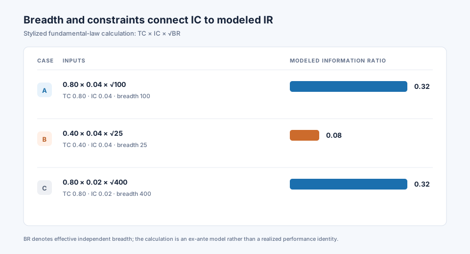
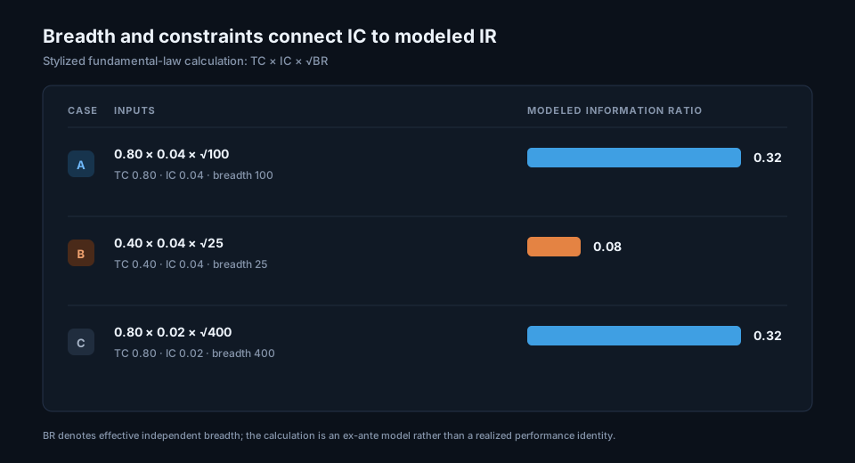
Cases A and B begin with the same IC, but reduced breadth and tighter transfer cut the modeled IR from \(0.32\) to \(0.08\). Case C has half the IC of Case A and four times the breadth, so the two have the same modeled IR under the stated transfer coefficient.
The relation is a planning model built on assumptions about independent forecasts, consistent definitions, portfolio optimization, and the covariance structure. It is not an accounting identity for realized rank IC and realized portfolio IR. Costs, estimation error, changing opportunity sets, and dependent decisions all affect the empirical result.
Statistical limitations
The familiar \(\sqrt{A}\) annualization is exact for the ratio under restrictive independent, identically distributed return assumptions. Serial correlation in active returns changes the appropriate time aggregation. Autocorrelation can arise from overlapping holdings, stale prices, illiquid assets, smoothed marks, or a slowly changing strategy. In those cases, mechanically multiplying a monthly ratio by \(\sqrt{12}\) can misstate the annual figure.
The ratio is also estimated with error. A short sample can produce a large positive or negative result by chance, while a very small tracking-error estimate can make the quotient unstable. Reporting mean active return, tracking error, observation count, sample dates, and a dependence-aware confidence interval makes the evidence easier to assess than the ratio alone.
Selecting the strongest IR after testing many factors, portfolio constraints, benchmarks, and start dates introduces selection bias. A later walk-forward or held-out period is needed to judge whether the selected construction retained its performance.
Common implementation mistakes
Comparing IC and IR as though they share a scale
IC is a bounded correlation between \(-1\) and \(1\). Information Ratio is an unbounded ratio of active return to tracking error. A value of \(0.05\) has a different meaning in each calculation.
Leaving the benchmark unspecified
Changing the benchmark changes every active return and therefore changes both the numerator and denominator of the Information Ratio. A cash benchmark, a broad market index, and a mandate-specific index answer different questions.
Misaligning the forecast target and portfolio result
A one-week cross-sectional IC and a monthly portfolio IR may be useful in the same research record, but they cannot be connected without the intervening refresh, holding, and aggregation rules. Currency, universe, and gross or net treatment must also agree.
Treating nominal opportunities as breadth
Correlated securities, overlapping forecast horizons, related factors, and persistent positions reduce effective breadth. Multiplying the number of securities by the number of dates usually overstates the independent decision count.
Calling ICIR an Information Ratio
ICIR summarizes a correlation history. Portfolio IR summarizes an active-return history. Use the full label in tables and APIs when both appear.
Reporting a gross ratio without implementation costs
Turnover, spreads, commissions, market impact, borrow expense, and financing can materially reduce active return. State gross and net values separately and record the cost model used for the net series.
Annualizing through serial dependence
The square-root rule assumes a return process that permits that aggregation. Inspect autocorrelation and use a dependence-aware estimate when active returns overlap or persist.
Dividing by negligible tracking error
A tiny denominator can generate a large, unstable ratio; zero tracking error makes it undefined. Always show the numerator and denominator beside the IR.
Relationship to adjacent measures
Mean IC magnitude describes the average strength of forecast ordering. IC reliability examines whether that mean is supported by enough appropriately adjusted evidence, and ICIR records consistency through the IC history. Those statistics remain attached to the forecast.
The Sharpe ratio uses return above a risk-free rate or cash reference divided by total return volatility. Information Ratio uses return relative to a portfolio benchmark divided by tracking error. The two coincide only in particular settings, such as a zero-beta strategy measured against cash under aligned return conventions.
Tracking errorTracking errorThe standard deviation of active return relative to a benchmark. is the denominator of the portfolio IR and can be useful on its own. Active share measures holdings-level distance from a benchmark, while tracking error measures return-level distance; portfolios with similar active share can have different tracking error because their active holdings have different covariances.
How StrategyNet keeps the evidence connected
StrategyNet records factor IC and ICIR with the signal version, eligible universe, observation time, forward-return horizon, lag, currency, coverage, and individual date-level observations. Candidate portfolios retain a separate record of weights, benchmark, constraints, risk estimates, trades, costs, active returns, and tracking error.
This separation allows the software to trace a forecast through portfolio construction without treating a signal statistic as a portfolio result. Researchers can compare the IC evidence with gross and net Information Ratios, inspect how constraints changed the position pattern, and determine whether breadth, transfer, risk, or implementation explains the difference. The result remains a reproducible research record for the user's chosen signal and portfolio specification.
Frequently asked questions
What benchmark should be used for Information Ratio?
Use the benchmark that represents the portfolio's stated mandate or opportunity set, and disclose it with the result. Replacing it with another index changes the measurement question.
Should Information Ratio be calculated gross or net of costs?
Both can be useful when clearly labeled. Gross IR isolates the modeled construction before implementation; net IR shows the return path after the declared cost assumptions or realized expenses.
What is a good Information Ratio?
There is no context-free threshold. The sample length, benchmark, frequency, serial dependence, tracking-error level, cost treatment, and selection process all affect interpretation. Review the numerator, denominator, confidence interval, and out-of-sample record.
Next reading
- From Information Coefficient to Portfolio Weights
- Should Information Coefficient Be Sector Neutral?
- Rolling ICIR: measuring the persistence of signal ranking
Sources
- Richard C. Grinold, “The Fundamental Law of Active Management”, The Journal of Portfolio Management, 1989.
- Roger Clarke, Harindra de Silva, and Steven Thorley, “Portfolio Constraints and the Fundamental Law of Active Management”, Financial Analysts Journal, 2002.
- CFA Institute, “The Sharpe Ratio and the Information Ratio”.
- Andrew W. Lo, “The Statistics of Sharpe Ratios”, Financial Analysts Journal, 2002.
This walkthrough is for research and educational purposes. It illustrates how strategynet.ai organizes signal evidence into factors and scenarios. It provides no recommendation, investment advice, or instruction to trade any security.
Back to Insights