From Information Coefficient to Portfolio Weights

Information coefficient reaches portfolio weights through a sequence of estimates. The signal is first calibrated into expected returns on a declared horizon. A portfolio model then combines those forecasts with covariance, constraints, current holdings, liquidity, and trading costs. IC supports the forecast estimate, but it does not supply a position size by itself.

This separation explains why a security with the highest signal rank may not receive the largest weight. Its forecast can be offset by high risk, strong correlation with existing positions, a sector limit, a concentration cap, or the cost of trading into the position. The complete mapping remains testable only when the signal, calibration, risk model, optimizer, and execution assumptions are all dated and versioned.

The signal-to-weight sequence

For security \(i\) in the point-in-time eligible universe \(U_t\), let \(f_{i,t}\) be the signal observed at time \(t\). Let \(R_{i,t\rightarrow t+h}^{(b)}\) be the forward return over horizon \(h\) in base currency \(b\). A date-level information coefficient measures the cross-sectional association between those fields:

\[\rho_t = \operatorname{corr}_{i\in U_t} \left( f_{i,t}, R_{i,t\rightarrow t+h}^{(b)} \right),\]

with ranks applied to both fields when the chosen convention is rank IC. The IC history establishes whether the signal carried repeatable ordering evidence under the registered universe, timing, and return definition.

Portfolio construction requires an expected-return forecastExpected returnThe conditional return estimate supplied to an allocation model. Realized returns can differ from the estimate.Open glossary entry → in units that can be combined with risk. Write the calibration as

\[\widehat\mu_{i,t} = g_t(f_{i,t}),\]

where \(g_t\) is estimated from information available before the portfolio date. It can be a cross-sectional slope, a quantile-return curve, a monotonic fit, or a shrunken combination of several estimates. The output \(\widehat\mu_{i,t}\) must use the same horizon and base currency as the risk and cost inputs.

Given expected returns \(\widehat\mu_t\), covariance matrix \(\widehat\Sigma_t\), risk-aversion parameter \(\lambda\), previous weights \(w_{t-1}\), and feasible set \(\mathcal W_t\), a cost-aware mean-variance problem can be written as

\[w_t^* = \underset{w\in\mathcal W_t}{\operatorname{argmax}} \left\{ \widehat\mu_t^{\mathsf T}w -\frac{\lambda}{2}w^{\mathsf T}\widehat\Sigma_t w -C_t(w-w_{t-1}) \right\}.\]

\(C_t\) represents the estimated cost of moving from current to proposed weights. The feasible set can include budget, gross leverage, long-only, shorting, concentration, sector, factor, currency, turnover, liquidity, and borrow constraints.

Without costs or constraints, and with an invertible covariance matrix, the solution is proportional to

\[w_t^* = \frac{1}{\lambda} \widehat\Sigma_t^{-1}\widehat\mu_t.\]

Even this simplified expression shows that expected returns enter through the inverse covariance matrix. Scores or IC values placed directly into weights skip the calibration and risk stages.

A special Pearson calibration

Suppose the signal has been standardized cross-sectionally so that \(\operatorname{Var}(z_t)=1\), and suppose the research uses Pearson IC. If the cross-sectional standard deviation of forward returns is \(\sigma_{R,t}\), then the fitted univariate slope is

\[\widehat\beta_t = \frac{\operatorname{Cov}(z_t,R_t)}{\operatorname{Var}(z_t)} = \widehat{\operatorname{IC}}_t\,\sigma_{R,t}.\]

After removing the common cross-sectional return mean, a simple linear forecast is therefore

\[\widehat\mu_{i,t} = \widehat{\operatorname{IC}}_t\,\sigma_{R,t}z_{i,t}.\]

This relation requires standardized scores, Pearson correlation, a linear conditional-mean model, and compatible estimates of IC and return dispersion. An estimated historical mean IC is normally shrunk to reflect its uncertainty rather than treated as known.

Rank IC does not provide a return scale in percentage points. A rank or percentile signal needs an empirical mapping from rank to subsequent return, such as walk-forward mean returns by quantile or a monotonic calibration curve. The rank IC remains useful evidence about ordering, while the calibration determines the economic magnitude passed to the optimizer.

Combining several factors

A composite forecast can combine user-defined factors, raw signals, and library factors in a matrix \(Z_t\):

\[\widehat\mu_t=Z_t\widehat\gamma_t.\]

Each column must be aligned to the same eligible securities and portfolio date. The coefficient vector \(\widehat\gamma_t\) can be estimated from cross-sectional slopes, forecast combinations, or a regularized model using only completed historical labels. Individual IC histories help diagnose the inputs, while joint calibration accounts for redundancy and interaction among them.

Adding two highly correlated factors at full strength can count much of the same evidence twice. Factor correlation, conditional IC, ablation tests, and walk-forward results help determine whether the combination adds independent forecast information. The final composite receives its own version and IC history.

A three-security numerical example

Consider a one-horizon synthetic example using Pearson calibration. The standardized signal is

\[z=(1.2,\ 0.6,\ -0.8)^{\mathsf T},\]

the estimated IC is \(0.05\), and forward-return dispersion is \(10\%\) over the same horizon. The calibrated expected returns are

\[\widehat\mu =0.05\times0.10\times z =(0.6\%,\ 0.3\%,\ -0.4\%)^{\mathsf T}.\]

Assume a diagonal covariance matrix with horizon volatilities of \(10\%\), \(5\%\), and \(10\%\). The unconstrained inverse-covariance signal is

\[\widehat\Sigma^{-1}\widehat\mu =(0.60,\ 1.20,\ -0.40)^{\mathsf T}.\]

Normalize this vector to 100% gross exposure. The resulting weights are \(27.3\%\), \(54.5\%\), and \(-18.2\%\). Security B has half the expected return of A and receives twice its optimized weight because its variance is one quarter as large under the example's diagonal risk model.

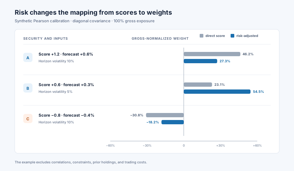
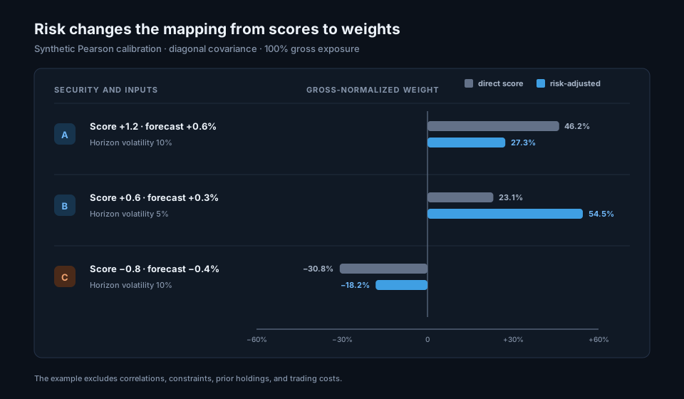
The example excludes correlations, position limits, current holdings, and costs. Adding those inputs can alter magnitudes further and can sometimes change a position's sign because one security can hedge risk contributed by another.

Python calculation

import numpy as np

standardized_score = np.array([1.2, 0.6, -0.8])
estimated_ic = 0.05
return_dispersion = 0.10
horizon_volatility = np.array([0.10, 0.05, 0.10])

expected_return = estimated_ic * return_dispersion * standardized_score
covariance = np.diag(horizon_volatility ** 2)

direct_weight = standardized_score / np.abs(standardized_score).sum()
unscaled_weight = np.linalg.solve(covariance, expected_return)
risk_adjusted_weight = unscaled_weight / np.abs(unscaled_weight).sum()

print("expected return", np.round(expected_return, 4))
print("direct weight", np.round(direct_weight, 4))
print("risk-adjusted weight", np.round(risk_adjusted_weight, 4))

# expected return       [ 0.0060  0.0030 -0.0040]
# direct weight         [ 0.4615  0.2308 -0.3077]
# risk-adjusted weight  [ 0.2727  0.5455 -0.1818]

The normalization fixes gross exposure for comparison. In a complete optimizer, \(\lambda\) and the portfolio constraints determine scale, while volatility targets or capital limits can provide an additional outer scaling step.

What positive, zero, and negative IC imply for weights

A reliably positive IC under the registered signal direction supports a positive calibration slope. The strength and uncertainty of the evidence affect how aggressively that slope is estimated or shrunk. Covariance and constraints still determine the final positions.

An IC near zero supplies little support for a nonzero return slope from that factor. Existing holdings, hedges, benchmark weights, and other signals can still produce nonzero portfolio positions because the portfolio contains more information than the single factor.

A negative IC means that the observed ordering ran against the registered direction. Reversing the signal after reading that result creates a new factor version and requires later validation. A stable negative relationship found in the research sample may motivate that new hypothesis; it does not retrospectively turn the original test into positive evidence.

Forecast uncertainty and shrinkage

Expected-return estimates are noisy, and mean-variance weights can respond sharply to small changes in them. Covariance estimates carry their own error, especially when the number of securities is large relative to the available history. Unconstrained inversion can amplify both sources of estimation error.

Common responses include shrinking expected returns toward zero or a prior, shrinking the covariance matrix, limiting turnover and concentration, imposing risk budgets, and solving a robust or resampled optimization problem. The shrinkage strength should be estimated or governed by a declared policy rather than chosen to improve the completed backtest.

Uncertainty can be propagated through the whole process by resampling completed forecast dates, recalibrating the signal, re-estimating covariance, and resolving the portfolio in each sample. The distribution of weights and portfolio results then reflects more of the estimation chain than an interval around mean IC alone.

Horizon alignment

The signal horizon governs the expected-return unit. A five-day IC cannot be combined directly with a one-year covariance matrix or a monthly cost estimate. Every field must be converted to a consistent horizon using assumptions that fit its time-series behavior.

IC decay helps identify when the forecast association appears, while turnover and costs help determine whether refreshing at that interval is implementable. Overlapping forward returns also reduce the effective number of independent calibration observations and must be reflected in uncertainty estimates.

Common implementation mistakes

Using rank IC as a percentage-return forecast

Rank IC is a dimensionless ordering statistic. A value of \(0.05\) does not mean a \(5\%\) expected return. Estimate a separate mapping from ranks or scores to returns in the correct units.

Setting weights equal to normalized scores

Direct score weights ignore security covariance, total risk, concentration, liquidity, existing holdings, and trading costs. They can serve as a transparent baseline, but they are a separate portfolio rule.

Calibrating on future or overlapping information

At each portfolio date, calibration may use only labels whose forward-return windows have completed. A five-day label observed one day ago is still unknown. The same embargo applies to model selection and shrinkage settings.

Combining incompatible horizons

Expected returns, covariance, costs, and turnover penalties must share a consistent time scale. Applying square-root scaling mechanically can fail when returns are serially dependent.

Ignoring factor redundancy

Correlated signals can repeat the same forecast information. Summing them as if they were independent can exaggerate expected returns and effective breadth.

Estimating and evaluating on the same sample

Calibration, factor selection, and optimizer settings chosen on the evaluation period bias the final result. Walk-forward testing must repeat every estimation step using the information set available at each date.

Hiding leverage and normalization

Weights can be normalized by net capital, gross exposure, volatility, or benchmark-relative risk. The selected denominator and any leverage cap need to be stated with the portfolio.

Omitting current holdings and costs

An optimizer that starts from zero each date can recommend excessive trading. Turnover penalties and implementation costs must depend on the move from actual or simulated prior holdings.

Treating sector-neutral IC as a portfolio constraint

Sector-neutral IC evaluates residual ranking evidence. The optimizer still needs explicit sector exposure bounds if the portfolio mandate requires them.

Relationship to adjacent measures

IC reliability describes the uncertainty around the mean forecast association. Rolling ICIR summarizes the stability of the recent IC history, and IC decay relates the association to forecast horizon. These diagnostics inform calibration and monitoring while leaving expected-return units to the fitted return model.

Portfolio Information Ratio evaluates the benchmark-relative return path after construction. The transfer coefficient in the fundamental law describes how constraints affect the passage from unconstrained forecasts to active positions. Effective breadth, risk, turnover, and costs help explain the remaining distance between forecast IC and realized portfolio IR.

Portfolio optimizationPortfolio optimizationThe selection of portfolio weights to maximize or minimize a stated objective subject to constraints.Open glossary entry → supplies the formal allocation problem. Tracking errorTracking errorThe standard deviation of active return relative to a benchmark., factor exposure, active share, turnover, drawdown, and implementation shortfall describe different properties of the resulting portfolio and its path.

How StrategyNet constructs the research record

Within StrategyNet, a user can combine raw signals, user-defined factors, and the factor library into a versioned composite. The software retains the input versions, timestamps, universe rules, transformations, factor correlations, and the composite's own walk-forward IC history.

The selected calibration converts that signal into expected returns. Portfolio construction then applies the dated covariance model, robust or tail-loss settings, exposure constraints, turnover policy, liquidity limits, current holdings, and cost assumptions. Each candidate set of weights remains linked to the exact inputs that produced it.

Walk-forward evaluation repeats the process through time and records gross and net returns, risk, drawdown, turnover, exposures, and benchmark-relative performance. The user's objective and constraints define the candidate portfolio; the software provides the calculation and evidence needed to compare those choices.

Frequently asked questions

Can IC be converted directly into a weight?

No. IC lacks return units and contains no security covariance, constraint, or cost information. It contributes to forecast calibration before the allocation problem is solved.

Can the highest-ranked security receive a smaller weight?

Yes. Higher risk, correlation with other positions, concentration limits, liquidity, or trading costs can reduce its allocation. Security B in the example receives the largest weight because its estimated variance is lower.

Can a positive forecast produce a short position?

It can in a multi-asset optimization. Correlation, hedging demand, factor constraints, benchmark-relative positions, and the forecasts for other securities all affect the joint solution.

How should rank IC be calibrated?

Estimate an out-of-sample relationship between ranks and subsequent returns, such as mean returns by score quantile or a regularized monotonic curve. Preserve the forecast horizon, lag, universe, currency, and missing-value rules.

How are several factors combined?

Align them point in time, normalize them under declared rules, measure their correlation and conditional contribution, estimate a joint or regularized calibration, and validate the resulting composite on later data.

Where does risk aversion enter?

The parameter \(\lambda\) sets the trade-off between expected return and variance in the stated objective. Gross exposure, volatility targets, and hard limits can also control the portfolio's scale.

What is the final validation target?

The whole walk-forward portfolio process must be evaluated after costs. Signal IC remains an important diagnostic, while portfolio return, risk, drawdown, turnover, exposure, capacity, and Information Ratio describe implementation.

Next reading

• Information Coefficient vs Information Ratio
• Should Information Coefficient Be Sector Neutral?
• Robust portfolio optimization beyond mean-variance

Sources

• Harry Markowitz, “Portfolio Selection”, The Journal of Finance, 1952.
• Richard C. Grinold, “The Fundamental Law of Active Management”, The Journal of Portfolio Management, 1989.
• Roger Clarke, Harindra de Silva, and Steven Thorley, “Portfolio Constraints and the Fundamental Law of Active Management”, Financial Analysts Journal, 2002.
• Richard O. Michaud, “The Markowitz Optimization Enigma: Is ‘Optimized’ Optimal?”, Financial Analysts Journal, 1989.
• Fischer Black and Robert Litterman, “Global Portfolio Optimization”, Financial Analysts Journal, 1992.