
How Does Information Coefficient Decay Across Forecast Horizons?
Information coefficient decay describes how a signal's association with subsequent returns changes across forecast horizons. Measuring that relationship helps researchers identify when a signal has been useful and choose horizons to investigate for trading and rebalancing.
This article holds a signal snapshot fixed and measures IC over several predeclared horizons. It explains cumulative and incremental return windows, shows why an IC curve can rise before declining, and discusses the uncertainty created by overlapping return observations.
Defining the horizon curve
Let \(f_{i,t}\) be the signal score for security \(i\) in the point-in-time eligible universe \(U_t\). For a cumulative horizon of \(h\) trading periods, define the base-currency simple return as
\[R_{i,t\rightarrow t+h}^{(b)} = \frac{P_{i,t+h}^{(b)}}{P_{i,t}^{(b)}}-1,\]
where the price series includes the stated corporate-action and distribution convention. The date-level rank IC at horizon \(h\) is
\[\rho_t(h) = \operatorname{corr}_{i\in U_t} \left( \operatorname{rank}(f_{i,t}), \operatorname{rank}(R_{i,t\rightarrow t+h}^{(b)}) \right).\]
Across \(T_h\) completed observation dates, the estimated horizon curve is
\[\widehat{\mu}_{IC}(h) = \frac{1}{T_h}\sum_{t=1}^{T_h}\rho_t(h), \qquad h\in\mathcal H,\]
where \(\mathcal H\) might be \(\{1,2,5,10,20\}\) trading days. Each point is a mean of cross-sectional correlations. The number of valid securities \(N_{t,h}\) and completed dates \(T_h\) should be reported because longer horizons can lose recent dates and securities with incomplete return labels.
Calendar time and trading time are distinct specifications. Five equity trading days, five calendar days and 120 continuous crypto hours can represent different information windows. Cross-asset research needs an explicit calendar and closing-time rule before those horizon values are compared.
A six-security example
The table holds one signal ranking fixed and compares three cumulative return horizons. Returns are synthetic and measured from the same observation time.
Synthetic signal ranks and cumulative forward returns
| Security | Signal rank | 1-day return | 5-day return | 20-day return |
|---|---|---|---|---|
| A | 1 | −1.4% | −2.0% | −0.8% |
| B | 2 | +0.2% | −0.8% | +1.5% |
| C | 3 | −0.5% | +0.1% | −1.7% |
| D | 4 | +0.6% | +1.9% | +2.2% |
| E | 5 | +1.7% | +1.2% | −0.2% |
| F | 6 | +1.2% | +2.6% | +0.7% |
With no tied ranks, Spearman correlation can be calculated from
\[\rho(h)=1-\frac{6\sum_{i=1}^{N}d_i(h)^2}{N(N^2-1)},\]
where \(d_i(h)\) is the difference between the signal rank and the return rank at horizon \(h\). The return-rank sequences are
\[\begin{aligned} 1\text{-day}:&\quad (1,3,2,4,6,5),\\ 5\text{-day}:&\quad (1,2,3,5,4,6),\\ 20\text{-day}:&\quad (2,5,1,6,3,4). \end{aligned}\]
Their rank IC values are \(0.886\), \(0.943\) and \(0.257\). In this example the ordering improves through day 5 and becomes much less informative by day 20. Six securities make the calculation inspectable; the sample is too small for statistical inference.
A simulation of delayed response and decay
The following simulation uses 240 independent synthetic observation dates and 400 securities per date. A latent signal contributes to standardized daily returns for the first five future days, with loadings of \(0.10\), \(0.08\), \(0.06\), \(0.04\) and \(0.02\). Later daily returns contain independent noise with no signal loading. The code computes cumulative-return rank IC at five horizons.
from math import sqrt
from random import Random
from statistics import mean, stdev

def rank(values):
    ordered = sorted(range(len(values)), key=values.__getitem__)
    result = [0] * len(values)
    for value_rank, index in enumerate(ordered, start=1):
        result[index] = value_rank
    return result

def spearman(x, y):
    rx, ry = rank(x), rank(y)
    midpoint = (len(x) + 1) / 2
    numerator = sum((a - midpoint) * (b - midpoint) for a, b in zip(rx, ry))
    denominator = sum((a - midpoint) ** 2 for a in rx)
    return numerator / denominator

rng = Random(17)
horizons = (1, 2, 5, 10, 20)
loadings = (0.10, 0.08, 0.06, 0.04, 0.02) + (0.0,) * 15
ic_by_horizon = {horizon: [] for horizon in horizons}

for _ in range(240):
    score = [rng.gauss(0, 1) for _ in range(400)]
    return_path = [
        [loadings[day] * value + rng.gauss(0, 1) for day in range(20)]
        for value in score
    ]
    for horizon in horizons:
        forward_return = [sum(path[:horizon]) for path in return_path]
        ic_by_horizon[horizon].append(spearman(score, forward_return))

for horizon, observations in ic_by_horizon.items():
    mean_ic = mean(observations)
    standard_error = stdev(observations) / sqrt(len(observations))
    print(horizon, round(mean_ic, 4), round(standard_error, 4))

# horizon  mean IC  ordinary standard error
# 1        0.0887   0.0033
# 2        0.1179   0.0032
# 5        0.1291   0.0032
# 10       0.0915   0.0033
# 20       0.0636   0.0032
The simulated draws are continuous, so the compact rank function needs no tie averaging. Empirical code should apply and record a consistent tie convention.
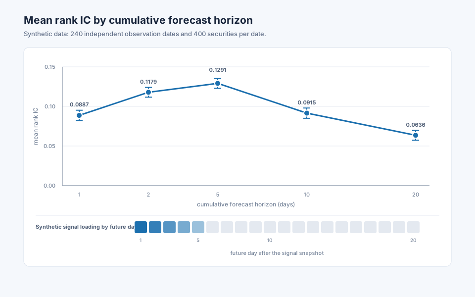
The simulation isolates one mechanism. Empirical observation dates are commonly dependent, and daily multi-period return labels overlap. Their confidence intervals require the dependence-aware treatment described in When Is an Information Coefficient Reliable?.
Cumulative horizons and incremental return buckets
A cumulative five-day IC asks whether the score at \(t\) ranks the complete return from \(t\) through \(t+5\). A cumulative ten-day IC repeats the calculation through \(t+10\), so the two labels share their first five days. This curve measures how well one signal snapshot orders the return accumulated by each endpoint.
An incremental, or bucket, IC asks when the information is expressed. For two endpoints \(h_1<h_2\), define
\[\rho_t(h_1,h_2) = \operatorname{corr}_{i\in U_t} \left( \operatorname{rank}(f_{i,t}), \operatorname{rank}(R_{i,t+h_1\rightarrow t+h_2}^{(b)}) \right).\]
For simple returns, the bucket return must preserve compounding:
\[R_{t+h_1\rightarrow t+h_2} = \frac{1+R_{t\rightarrow t+h_2}} {1+R_{t\rightarrow t+h_1}}-1.\]
Subtracting the two cumulative simple returns is only an approximation. With log returns, the corresponding cumulative values can be subtracted exactly.
Both views are useful. Cumulative IC answers how well the original ranking predicts the return available by an endpoint. Bucket IC identifies whether the association is concentrated early, continues through later periods, or reverses after the initial response.
Why an IC curve can rise before it falls
The forecast takes time to enter prices
Some inputs are absorbed gradually because investors update at different speeds, liquidity is uneven, or the economic effect arrives through later cash-flow information. Early return windows then contain only part of the relationship.
Predictive return accumulates during an active interval
When several consecutive return periods share the signal direction, the cumulative association can strengthen through that interval. The simulation uses this structure during its first five days.
Unrelated variation accumulates later
Once the signal contribution has largely arrived, additional return periods add market, sector and security-specific movements. Those movements can change the final ordering and reduce cumulative rank IC.
The relationship reverses
A short-lived continuation effect can be followed by price correction or mean reversion. Incremental bucket IC may become negative even while the longer cumulative IC remains positive because the earlier return is still included.
The evaluated sample changes with the horizon
Longer horizons exclude more recent observation dates and can lose securities through delistings, stale prices or missing data. A change in membership can move the curve even when the underlying forecast relationship is unchanged.
Summaries derived from the curve
For a signal registered with a positive direction, the peak measured horizon is
\[h_{\mathrm{peak}} = \underset{h\in\mathcal H}{\operatorname{argmax}} \ \widehat{\mu}_{IC}(h).\]
Relative retention after that peak can be written as
\[D(h;h_{\mathrm{peak}}) = \frac{\widehat{\mu}_{IC}(h)} {\widehat{\mu}_{IC}(h_{\mathrm{peak}})}, \qquad h\ge h_{\mathrm{peak}}.\]
In the simulation, 20-day retention is \(0.0636/0.1291\approx49\%\). The ratio is unstable when the peak estimate is close to zero, and its uncertainty should be evaluated from the joint horizon estimates.
A decay half-life is sometimes reported as the first post-peak horizon at which a smoothed curve falls below half its peak. That summary needs a declared interpolation and smoothing rule. Sparse or non-monotonic curves may have no well-defined half-life, in which case the estimated points are more informative than a fitted exponential.
Statistical treatment of multiple horizons
When an \(h\)-day forward return is recalculated every day, adjacent labels share up to \(h-1\) daily return periods. The time series \(\rho_t(h)\) can therefore be serially correlated. An ordinary standard error based on \(T_h\) independent dates can understate uncertainty when those autocovariances are positive.
A pre-specified heteroskedasticity and autocorrelation consistent estimator or a suitable block bootstrap can account for this dependence. The horizon gives useful information for choosing an initial lag or block length, while signal persistence and market regimes may extend dependence beyond the mechanical overlap.
The curve also represents a family of tests. Selecting the largest IC from 20 horizons and reporting its unadjusted confidence interval omits the selection step. A practical research design declares a compact, economically motivated horizon grid, retains all results, and evaluates the chosen horizon in a later walk-forward period.
Common implementation mistakes
Moving the signal timestamp with each endpoint
An IC horizon curve holds the signal at \(t\) fixed. Updating the signal at each future date measures a sequence of new forecasts and answers a different question.
Mixing cumulative and bucket returns
The labels should state whether \(5D\) means \(t\rightarrow t+5\) or a later bucket such as \(t+1\rightarrow t+5\). Otherwise two distinct decay profiles can be presented as the same result.
Letting availability rules change silently
Long-horizon returns need delisting treatment and sufficient price history. Report \(N_{t,h}\) and \(T_h\), and compare a common-date sample when changing coverage appears to drive the result.
Treating overlapping dates as independent
Daily calculation adds resolution to the curve. Multi-day labels remain dependent, so the uncertainty method should reflect the return window and observed IC autocorrelation.
Annualizing correlation
IC is dimensionless. Multiplying a five-day IC by an annualization factor leaves it dimensionless and creates no valid comparison with an annual return or a portfolio information ratio.
Equating the peak with a mandatory holding period
The peak summarizes one fixed signal snapshot. A live strategy can refresh scores, maintain overlapping cohorts, impose turnover limits and trade only when expected improvement exceeds cost. Its rebalance and holding rules need a portfolio-level test.
Relationship to adjacent measures
Mean IC magnitude describes the strength of association at one stated horizon. The decay curve repeats that estimate across a controlled horizon grid. Rolling ICIR instead follows the stability of IC through calendar time for a chosen horizon. One study can therefore report a horizon curve for forecast timing and a rolling ICIR series for historical stability.
Signal rank autocorrelation measures how similar the factor's own security ranking remains between observation dates. IC decay measures how one ranking relates to returns at later endpoints. A slowly changing factor can lose its predictive relationship quickly, and a rapidly changing factor can have a useful multi-day cumulative IC.
Turnover measures the trading implied by updated portfolio weights. It connects the forecast horizon with implementation cost, but it depends on score changes, construction rules, constraints and rebalance policy in addition to IC decay.
How horizon decay enters StrategyNet evaluation
StrategyNet evaluates a registered factor version across declared forecast horizons while retaining the observation timestamp, execution lag, universe, currency, coverage and return-label convention. The record contains date-level IC, mean IC, uncertainty and valid counts for each endpoint, together with incremental buckets when the timing of the response needs to be isolated.
This evidence informs the temporal contract used in signal and strategy tests: how frequently a score can be refreshed, how long its forecast remains useful, and which return windows deserve portfolio evaluation. Candidate portfolios are then compared under their actual rebalance schedule, overlapping positions, constraints, turnover and estimated costs. That stage determines whether the measured decay profile can be implemented economically.
Frequently asked questions
What is the best forecast horizon?
The most useful horizon has stable out-of-sample evidence and fits the intended decision frequency, liquidity and costs. The largest in-sample mean IC is a candidate that still needs uncertainty, multiple-testing and portfolio checks.
Can IC increase at longer horizons?
Yes. A relationship can take several periods to appear in prices, so cumulative IC may rise before reaching its peak. Incremental bucket IC helps identify where the additional association occurs.
What does a negative long-horizon IC mean?
The original ranking was inversely associated with returns at that endpoint. It can reflect reversal, a changing regime, a different evaluated sample or sampling variation. The bucket curve shows whether the negative association arose late in the window.
Should forward-return windows overlap?
Overlapping windows retain a daily view of the curve and are valid when their dependence is handled in the uncertainty estimate. Non-overlapping samples offer simpler dependence at the cost of fewer observation dates.
Is IC decay the same as factor autocorrelation?
No. Factor autocorrelation compares the signal ranking with its own later ranking. IC decay compares the original signal ranking with forward-return rankings at several endpoints.
Does a five-day IC peak imply weekly rebalancing?
It provides evidence about the cumulative forecast horizon. Rebalancing also depends on how often new scores arrive, score persistence, turnover, capacity, constraints and costs. Those elements belong in the candidate portfolio test.
Next reading
- When Is an Information Coefficient Reliable?
- Rolling ICIR: measuring the persistence of signal ranking
- Information Coefficient vs Hit Rate
Sources
- Charles Spearman, “The Proof and Measurement of Association between Two Things”, The American Journal of Psychology, 1904.
- Alphalens API documentation, including forward-return periods and mean Spearman information coefficient.
- Whitney K. Newey and Kenneth D. West, “A Simple, Positive Semi-definite, Heteroskedasticity and Autocorrelation Consistent Covariance Matrix”, Econometrica, 1987.
- Matthew Richardson and James H. Stock, “Drawing Inferences From Statistics Based on Multi-Year Asset Returns”, Journal of Financial Economics, 1989.
- SciPy
spearmanrdocumentation
This walkthrough is for research and educational purposes. It illustrates how strategynet.ai organizes signal evidence into factors and scenarios. It provides no recommendation, investment advice, or instruction to trade any security.
Back to Insights