
Combining Short- and Long-Horizon Risk Models
Short- and long-history covariance estimates capture different aspects of portfolio risk. A short history responds quickly to changing volatility and correlation; a longer history estimates those relationships from more observations. This walk-forward study compares fixed and changing covariance blends with separate risk limits under both models.
Separate limits produced the strongest risk control in this sample. Realized volatility was 10.30%, compared with 10.93% for the equal blend and 10.97% for the changing weight; maximum drawdown was 19.98%, compared with 22.29% and 22.80%, respectively. Both the calibration-selected fixed weight and the changing weight produced higher realized volatility than the equal blend.
The comparison uses gross results from one eight-factor panel and sixteen reporting rebalances. Within that sample, retaining each model's risk limit provided more protection than estimating a weight to average the models.
The common-universe combination
Let \(\Sigma_{S,t}\) be a short-window covariance and \(\Sigma_{L,t}\) a long-window covariance available at rebalance \(t\). Both matrices describe the same \(N\) factor returns in the same order and daily units. A convex combination is
\[\Sigma_t(\lambda_t) = (1-\lambda_t)\Sigma_{S,t} + \lambda_t\Sigma_{L,t}, \qquad 0\leq\lambda_t\leq1.\]
The parameter \(\lambda_t\) is the weight on the 126-observation model in this article. Zero uses only the 42-observation covariance, one uses only the longer history, and \(\lambda_t=0.5\) gives both matrices equal weight. Positive semidefiniteness is preserved because the weights are non-negative and sum to one.
For any fixed portfolio \(w\), the predicted variance is linear in the model weight:
\[w^{\mathsf T}\Sigma_t(\lambda_t)w = (1-\lambda_t)w^{\mathsf T}\Sigma_{S,t}w + \lambda_t w^{\mathsf T}\Sigma_{L,t}w.\]
Volatility follows after taking the square root. A 50% covariance blend does not imply the arithmetic average of the two volatility forecasts.
A two-asset calculation
Suppose the short and long models estimate annual covariance as
\[\Sigma_S= \begin{bmatrix} 0.0400 & 0.0180\\ 0.0180 & 0.0225 \end{bmatrix}, \qquad \Sigma_L= \begin{bmatrix} 0.0225 & 0.0090\\ 0.0090 & 0.0169 \end{bmatrix}.\]
With 35% on the long model,
\[\Sigma(0.35) =0.65\Sigma_S+0.35\Sigma_L = \begin{bmatrix} 0.033875 & 0.014850\\ 0.014850 & 0.020540 \end{bmatrix}.\]
For \(w=(0.5,0.5)^{\mathsf T}\), the short and long models forecast 15.69% and 11.98% volatility. The combined variance is
\[w^{\mathsf T}\Sigma(0.35)w =0.65(0.024625)+0.35(0.014350) =0.02102875,\]
which gives 14.50% volatility. Directly averaging the two volatility figures would give 14.39%, a different quantity.
import numpy as np

def combine_covariances(short_cov, long_cov, long_weight):
    if not 0.0 <= long_weight <= 1.0:
        raise ValueError("long_weight must lie in [0, 1]")
    combined = (
        (1.0 - long_weight) * short_cov
        + long_weight * long_cov
    )
    return 0.5 * (combined + combined.T)

def predicted_volatility(weight, covariance):
    variance = weight @ covariance @ weight
    return np.sqrt(max(float(variance), 0.0))
A constructive allocation example
To see the portfolio effect without tying the calculation to one historical period, consider three investable factors with annual expected returns of 12%, 9%, and 7%. Suppose their short-window covariance is
\[\Sigma_S= \begin{bmatrix} 0.0400 & 0.0120 & 0.0060\\ 0.0120 & 0.0225 & 0.0045\\ 0.0060 & 0.0045 & 0.0144 \end{bmatrix},\]
while the longer estimate is
\[\Sigma_L= \begin{bmatrix} 0.0256 & 0.0080 & 0.0040\\ 0.0080 & 0.0196 & 0.0035\\ 0.0040 & 0.0035 & 0.0121 \end{bmatrix}.\]
For a fully invested minimum-variance allocation, with short sales allowed in the formula but unnecessary in this example,
\[w^*(\Sigma) = \frac{\Sigma^{-1}\mathbf 1} {\mathbf 1^{\mathsf T}\Sigma^{-1}\mathbf 1}.\]
Illustrative minimum-variance allocations
| Covariance used | Factor weights | Expected return | Predicted volatility |
|---|---|---|---|
| Short model | 8.3%, 30.8%, 61.0% | 8.03% | 10.32% |
| Long model | 16.0%, 26.7%, 57.4% | 8.33% | 9.23% |
| 35% long-model pool | 10.4%, 29.6%, 60.1% | 8.11% | 9.97% |
def minimum_variance(covariance):
    one = np.ones(covariance.shape[0])
    precision_times_one = np.linalg.solve(covariance, one)
    return precision_times_one / (one @ precision_times_one)

pooled = combine_covariances(short_cov, long_cov, 0.35)
weight = minimum_variance(pooled)
expected_return = weight @ np.array([0.12, 0.09, 0.07])
The positive expected returns make the example resemble a portfolio a user might consider deploying, and they are assumptions supplied solely for this calculation. The pooled covariance changes the risk estimate and, through that estimate, the allocation. This distinction matters when a historical factor panel has a poor return period: covariance quality can still be evaluated, but a risk model should receive neither credit nor blame for an expected-return forecast supplied elsewhere in the process.
How the weight was learned
Every candidate covariance was scored on returns observed after the covariance date. If \(r_{u}\) is an \(N\)-factor return vector in the next holding interval, the zero-mean Gaussian negative log predictive density is
\[\ell_u(\lambda) = \frac{1}{2} \left[ N\log(2\pi) +\log|\Sigma_t(\lambda)| +r_u^{\mathsf T}\Sigma_t(\lambda)^{-1}r_u \right].\]
Lower values indicate a better density forecast. The static weight was chosen once from a grid \(\{0,0.05,\ldots,1\}\) using only the six completed calibration intervals:
\[\widehat\lambda_{\mathrm{static}} = \arg\min_{\lambda} \frac{\sum_{j=1}^{6}n_j\overline\ell_j(\lambda)} {\sum_{j=1}^{6}n_j},\]
where \(n_j\) is the number of daily observations in interval \(j\). This selected \(\widehat\lambda_{\mathrm{static}}=0.35\) under the Gaussian score.
A Student-\(t\) density with five degrees of freedom was retained as a heavy-tailed diagnostic. It selected \(\lambda=0.70\) from exactly the same calibration observations. That 35-percentage-point difference is important: an estimated model weight inherits the assumptions of the scoring distribution and should not be presented as though the data identified one unambiguous number.
The changing weight
At each reporting rebalance, the dynamic method rescored the grid using only holding intervals that had already ended. Older intervals received an exponentially declining weight with a six-rebalance half-life, and a quadratic penalty discouraged movement away from the previous model weight:
\[\widehat\lambda_t = \arg\min_{\lambda} \left\{ \widetilde L_t(\lambda) + \gamma(\lambda-\widehat\lambda_{t-1})^2 \right\}, \qquad \gamma=1.\]
Here \(\widetilde L_t\) is the discounted mean Gaussian score, normalized by its cross-grid standard deviation at that decision date. A move across the full 0–1 weight range therefore costs one cross-grid score standard deviation. The penalty regulates changes in the risk-model weight; it is distinct from a portfolio turnover penalty on the factor holdings.
def choose_dynamic_weight(score_history, previous, grid, gamma=1.0):
    # score_history contains completed holding intervals only
    ages = np.arange(len(score_history) - 1, -1, -1)
    discount = 0.5 ** (ages / 6.0)
    score = np.average(score_history, axis=0, weights=discount)
    scale = max(float(np.std(score)), 1e-12)
    normalized = (score - score.min()) / scale
    objective = normalized + gamma * (grid - previous) ** 2
    return float(grid[np.argmin(objective)])
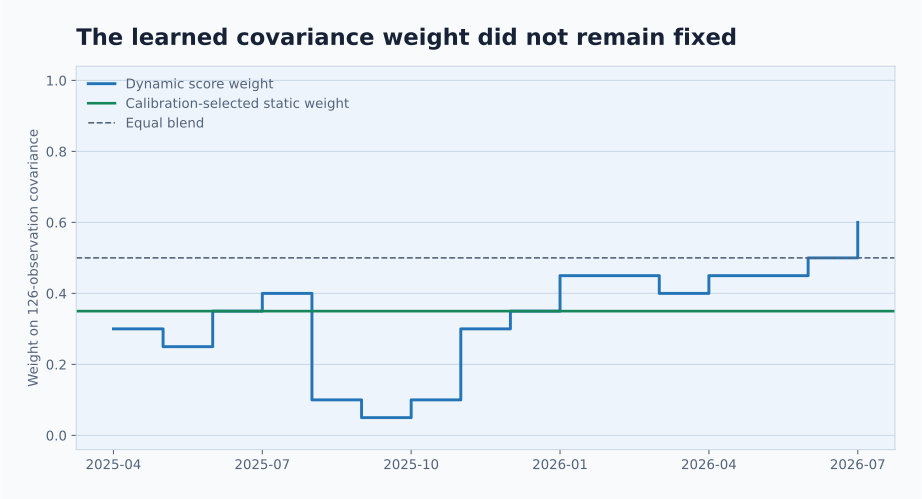
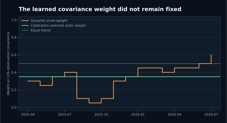
The reporting weight averaged 0.344, close to the static estimate, but its path ranged from 0.05 to 0.60. Its mean absolute change was 0.08 per rebalance.
The portfolio experiment
The factor panel is the same predefined panel used in the preceding multiple-risk-model study: eight registered long-short factor spreads covering momentum, reversal, volatility, intraday price relationships, and a technical composite. The common history runs from 3 April 2024 through 16 July 2026, with average daily security coverage between about 1,310 and 1,342 names.
Covariances used 25% diagonal shrinkage. Expected factor returns came from the previous 63 observations, portfolios were recomputed every 21 common observations, weights were non-negative and fully invested, and no factor could exceed 35%. A pooled covariance limit was set at 110% of contemporaneous equal-weight risk under that covariance. The separate-limit control applied the same relative calculation independently to the short and long matrices.
Six rebalances from October 2024 through March 2025 formed the calibration period. The reporting sample begins on 7 April 2025 and contains 320 daily observations across sixteen rebalances. Every forecast, covariance, model weight, and portfolio weight stops before the return it is evaluated against.
Historical risk outcomes
Walk-forward risk results, gross of transaction costs
| Risk-model construction | Annualized volatility | Maximum drawdown | Mean one-way turnover |
|---|---|---|---|
| 42-observation covariance | 11.01% | 22.42% | 41.64% |
| 126-observation covariance | 10.93% | 21.89% | 39.95% |
| Equal covariance blend | 10.93% | 22.29% | 40.31% |
| Gaussian calibration weight, 0.35 long | 10.97% | 22.51% | 40.83% |
| Changing Gaussian score weight | 10.97% | 22.80% | 40.88% |
| Separate short and long limits | 10.30% | 19.98% | 40.11% |
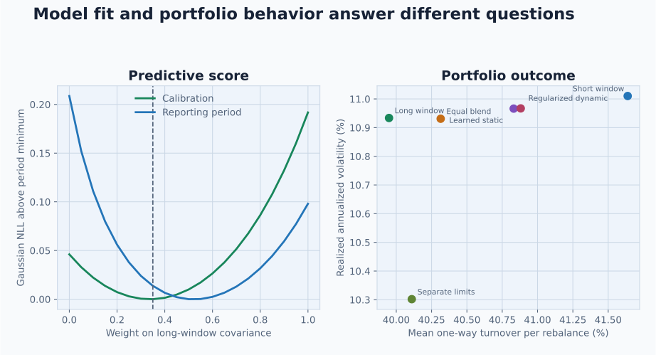
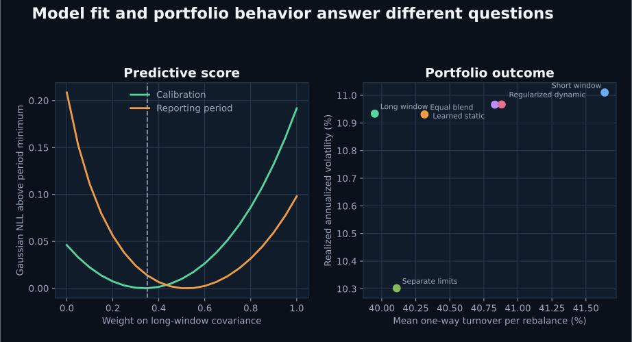
The pooled methods formed a tight cluster. Their annualized volatility ranged from 10.93% to 11.01%, while mean one-way turnover ranged from 39.95% to 41.64%. Learning a covariance weight did not produce a lower-risk portfolio: the fixed 0.35 rule and the changing rule both recorded 10.97% volatility, and the latter had the largest drawdown among the six constructions.
The predictive scores tell a compatible story. During the reporting period, the Gaussian score reached its minimum at \(\lambda=0.50\); the weight chosen from calibration, \(0.35\), produced a slightly worse mean score of -24.141 against -24.154 for the equal blend. The dynamic path scored -24.109. The numbers are negative because return covariances in daily units create densities greater than one. Their relative values carry the interpretation.
Forecast calibration and the separate-limit result
For each holding interval, the study compared squared realized portfolio returns with the variance forecast available at the preceding rebalance. A volatility-calibration ratio of one means that aggregate realized root-mean- square return matched predicted volatility; values above one indicate underprediction.
The short model's ratio was 1.044, the equal blend's 1.067, and the long model's 1.105. Recent covariance therefore tracked the scale better in this sample, even though using it alone did not produce the portfolio with the lowest realized volatility. The selected holdings and the covariance's density fit are related, but they are not the same evaluation object.
The dual construction has no single pooled covariance, so assigning it a Gaussian density score would invent a model that the optimizer never used. Its calibration diagnostic instead takes the greater of the short- and long-model variance forecasts for the chosen portfolio; the resulting volatility ratio was 0.982. Both named limits remained available to explain why a holding was accepted or rejected.
This approach reduced realized volatility by 0.63 percentage point relative to the long model and the equal blend, with essentially unchanged turnover. The trailing expected-return rule used by the historical experiment failed during the reporting period: annualized gross returns ranged from -17.91% to -15.66% across the six methods. That adverse outcome is retained in the record because removing it would overstate the evidence, although it is secondary to the risk question tested here. The result supports a risk-control comparison and no positive expected-return claim.
Why the learned weight failed to improve this portfolio
Only six calibration rebalances were available, and the disagreement between Gaussian and Student-\(t\) selection shows that the apparent optimum was not stable across plausible predictive distributions. The Gaussian surface was also fairly shallow near its minimum; small changes in score moved the selected grid point without supplying a correspondingly large change in portfolio risk.
Portfolio constraints further weaken the connection between matrix fit and realized risk. Position caps, the expected-return vector, and the relative risk limit determine which covariance directions the optimizer actually uses. A matrix can improve average density fit while making little difference along the directions carried by the selected portfolio. Recent decision-focused covariance research addresses this problem directly by training or validating estimators against the portfolio decision, although that extra flexibility requires a larger, carefully nested sample.
The dynamic penalty sensitivity did not reverse the result. Penalties of 0.25, 1, and 4 produced annualized volatility of 10.94%, 10.97%, and 10.96%; their maximum drawdowns were 22.41%, 22.80%, and 23.03%. In this sample, a smoother or more responsive model-weight path could not match the protection supplied by two explicit limits.
Common implementation mistakes
Selecting the weight on the reporting period
The reporting-period Gaussian optimum was 0.50, but it is an oracle diagnostic. Using it as though it had been known on 7 April 2025 would leak future returns into every subsequent portfolio.
Combining different units or asset orders
Daily covariance cannot be averaged with an annualized matrix, and columns must be reconciled by stable factor or security identifiers. Matching row numbers or display labels is insufficient.
Treating the scoring rule as a neutral detail
Gaussian and five-degree-of-freedom Student-\(t\) scores selected 0.35 and 0.70 from the same calibration sample. Distributional assumptions belong in the reported method and sensitivity analysis.
Letting the dynamic rule chase the latest interval
Short performance histories can generate sharp weight changes from noise. A forgetting schedule, change penalty, weight bounds, minimum history, and a fixed control should be declared before the reporting results are examined.
Assuming a pooled limit preserves both component limits
Low modeled risk under one covariance can offset high risk under the other. When each model represents a limit that must be honored, apply both constraints and record their slack separately.
Ranking matrices without evaluating the downstream portfolio
Predictive density, covariance-element loss, condition number, variance calibration, realized portfolio volatility, drawdown, concentration, and turnover answer different questions. The validation set should include the ones that match the model's intended use.
Relationship to adjacent methods
This experiment uses arithmetic covariance pooling, which preserves positive semidefiniteness and gives a transparent interpretation to \(\lambda\). Precision pooling averages inverse covariances, while log-Euclidean and Bures–Wasserstein means use different geometry on positive-definite matrices. Those constructions can be tested later, but a mathematically elegant average still needs a portfolio-aligned validation loss.
Covariance shrinkageCovariance shrinkageThe combination of a responsive covariance estimate with a more stable target to reduce estimation error and improve numerical conditioning.Open glossary entry → is closely related. The short model can be read as a responsive estimate and the long model as a target, although both covariances here already receive diagonal shrinkage before they are combined. Multiple-target shrinkage extends the same idea to several matrices.
Separate limits retain disagreement instead of reducing it to one matrix. That can be valuable when a recent statistical estimate, a long-run model, and a fundamental or stress model express risks that the mandate wants to monitor individually. It also makes the cost visible: every added constraint can reduce forecast exposure or render the feasible set too restrictive.
How this enters portfolio evaluation
A deployable risk-model combination should store the short and long covariance versions, the selected weight, every completed score used in selection, the previous weight, the change penalty, and the resulting portfolio-risk forecast. The portfolio record should retain the fixed-weight and separate-limit controls alongside realized variance, drawdown, concentration, and holdings turnover.
The present evidence does not justify replacing the separate-limit control with learned covariance weights. A larger nested study can add multiple factor panels and market regimes, tune the score and change penalty inside an inner validation loop, then test the frozen rule in an untouched outer period. Transaction costs remain outside this experiment and must be included before a method with materially different holdings turnover is considered operational.
Frequently asked questions
Should short- and long-window covariances always receive equal weight?
No. Equal weighting is a strong control because it uses no estimated model weight, and it performed well on predictive score in this sample. A different weight may be supported by a longer nested history or by a model designed for a specific decision.
Why not update the weight every day?
The covariance and portfolio were evaluated on 21-observation holding intervals. Daily weight updates would create a different experiment with more overlapping feedback, greater estimation noise, and potentially much more trading.
Is the Student-\(t\) selection preferable because financial returns have heavy tails?
It is a plausible diagnostic, but its degrees of freedom, scale convention, and portfolio consequence still require out-of-sample validation. Here it revealed that the calibration weight was sensitive to the assumed density.
Can the models use different factors or symbols?
A direct matrix average requires a common ordered universe. Partial overlap needs an explicit transfer calibration with held-out shared symbols, while disjoint universes require synchronized bridge factors or another identified source of cross-block covariance.
Did the changing weight reduce portfolio turnover?
No. Mean one-way holdings turnover was 40.88%, compared with 40.31% for the equal blend and 39.95% for the long model. The rule penalized changes in the covariance weight; it did not place transaction costs in the allocation objective.
Continue reading
- Covariance Shrinkage in Factor Risk Models
- When Does a Second Risk Model Improve Portfolio Construction?
- How Do Multiple Risk Models Enter Portfolio Construction?
Sources
- Luiz Koodi Hotta, Carlos Trucíos, Alexandre Rubesam, and André Alves Portela Santos, “Combining Covariance Forecasts for Large-Dimensional Portfolio Optimization”, 2026 working paper. Compares ten covariance estimators and five combination strategies in constrained portfolios containing as many as 1,000 equities.
- Thomas Conlon, John Cotter, and Iason Kynigakis, “Asset Allocation with Factor-Based Covariance Matrices”, European Journal of Operational Research, 2025. Evaluates static and dynamic factor-covariance specifications through minimum-variance portfolios and transaction-cost-adjusted outcomes.
- Juchan Kim, Inwoo Tae, and Yongjae Lee, “Estimating Covariance for Global Minimum Variance Portfolio: A Decision-Focused Learning Approach”, 2025 preprint. Shows why covariance prediction loss and downstream portfolio loss can rank estimators differently.
- Jorge Guijarro-Ordonez, Misha van Beek, and Amandeep Dhaliwal, “A Simple Responsive Covariance Matrix Forecaster for Multiple Horizons and Asset Classes”, revised 2025 working paper. Develops feature-dependent linear blends for stable multi-horizon covariance forecasts.
- Yijie Wang, Hao Gao, Campbell R. Harvey, Yan Liu, and Xinyuan Tao, “Machine Learning Meets Markowitz”, NBER Working Paper 34861, 2026. Provides a recent decision-focused account of why predictive precision should be evaluated through the investor's actual constraints and objective.
This walkthrough is for research and educational purposes. It illustrates how strategynet.ai organizes signal evidence into factors and scenarios. It provides no recommendation, investment advice, or instruction to trade any security.
Back to Insights