
How Do Multiple Risk Models Enter Portfolio Construction?
Portfolio construction can use several risk models to account for uncertainty about future covariance. Models based on different histories or assumptions may identify different concentrations in the same holdings, giving the portfolio manager several views of the proposed allocation's risk.
This article explains how to combine those views through covariance averaging, separate penalties or limits, and worst-model protection. The worked examples show how each choice changes the optimizer's treatment of model disagreement.
Risk under each model
Let \(\mathbf w\) be portfolio weights and \(\mathbf b\) benchmark weights. Active weights are
\[\mathbf a=\mathbf w-\mathbf b.\]
For risk model \(m\) with positive-semidefinite covariance matrix \(\Sigma_m\), predicted active risk is
\[\sigma_m(\mathbf a) = \sqrt{\mathbf a^{\mathsf T}\Sigma_m\mathbf a}.\]
Every model must describe the same assets, currency, return frequency, and annualization convention before these numbers can be compared. Coverage gaps and differing security mappings need explicit treatment; silently dropping a position from one covariance matrix reduces its reported risk.
Four ways to combine the models
Blend the covariance matrices
Choose non-negative weights \(\gamma_m\) that sum to one and form
\[\overline\Sigma = \sum_{m=1}^{M}\gamma_m\Sigma_m.\]
The optimizer then uses one covariance matrix. This is computationally simple and preserves convexity. It also permits low risk under one model to offset high risk under another in the weighted average.
Penalize every model in the objective
A quadratic objective can include a weighted sum of predicted variances:
\[\max_{\mathbf a\in\mathcal A} \left\{ \boldsymbol\alpha^{\mathsf T}\mathbf a -\frac{1}{2} \sum_{m=1}^{M}\lambda_m \mathbf a^{\mathsf T}\Sigma_m\mathbf a \right\}.\]
Algebraically this is a covariance blend with weights determined by the \(\lambda_m\) values, although the coefficients may be easier to interpret as separate risk prices.
Impose a risk limit under each model
Separate limits require
\[\sqrt{\mathbf a^{\mathsf T}\Sigma_m\mathbf a} \le \tau_m, \qquad m=1,\ldots,M.\]
Each quadratic risk limit is a second-order cone constraint after factoring the covariance matrix. This construction gives a direct guarantee under every included model. The limits can differ when the models have distinct calibration or mandate roles.
Minimize the largest modeled risk
A minimax formulation introduces \(z\) and solves
\[\min_{\mathbf a,z}\ z \quad\text{subject to}\quad \mathbf a^{\mathsf T}\Sigma_m\mathbf a\le z, \quad m=1,\ldots,M,\]
along with the portfolio constraints and, where required, an expected-return target. The result controls the model that regards a candidate portfolio most severely.
What each construction guarantees
| Construction | Main setting | Direct guarantee under every model |
|---|---|---|
| Covariance blend | Model weights γ | No |
| Weighted risk penalties | Risk prices λ | No |
| Separate risk limits | Risk caps τ | Yes |
| Worst-model objective | Return target or risk trade-off | Yes, for the modeled maximum |
A two-bet example
Consider two active positions with expected returns
\[\boldsymbol\alpha = \begin{bmatrix}1.0\\0.8\end{bmatrix}.\]
Two covariance models reverse which position they regard as risky:
\[\Sigma_1 = \begin{bmatrix}1&0\\0&9\end{bmatrix}, \qquad \Sigma_2 = \begin{bmatrix}9&0\\0&1\end{bmatrix}.\]
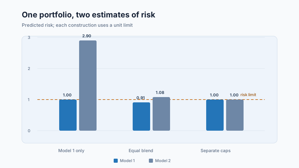
First maximize expected return subject only to \(\mathbf a^{\mathsf T}\Sigma_1\mathbf a\le1\). The solution is approximately \((0.966,0.086)\). It uses the full risk allowance under model 1, while model 2 assigns risk of 2.90 to the same position.
An equal blend gives \(\overline\Sigma=5I\). Applying a unit risk limit to the blend produces \((0.349,0.279)\). Its blended risk is exactly 1, but its risks under the component models are 0.91 and 1.08. The average satisfies its limit while model 2 does not.
Requiring unit risk under both models gives \((0.316,0.316)\). Both constraints bind, and the expected return is 0.569. The equal-blend solution has slightly higher expected return of 0.573 because it permits model 2 risk to exceed one.
Three constructions for the same expected-return vector
| Construction | Active weights | Risk under model 1 | Risk under model 2 | Expected return |
|---|---|---|---|---|
| Model 1 only | (0.966, 0.086) | 1.000 | 2.900 | 1.035 |
| Equal covariance blend | (0.349, 0.279) | 0.908 | 1.084 | 0.573 |
| Separate unit caps | (0.316, 0.316) | 1.000 | 1.000 | 0.569 |
import numpy as np

alpha = np.array([1.0, 0.8])
sigma_1 = np.diag([1.0, 9.0])
sigma_2 = np.diag([9.0, 1.0])

def risk(weight, covariance):
    return np.sqrt(weight @ covariance @ weight)

# A fine angular grid keeps the example independent of an optimization package.
theta = np.linspace(0.0, np.pi / 2.0, 20001)
direction = np.column_stack([np.cos(theta), np.sin(theta)])
blend = 0.5 * sigma_1 + 0.5 * sigma_2

def boundary(covariances):
    scales = []
    for covariance in covariances:
        variance = np.einsum("ij,jk,ik->i", direction, covariance, direction)
        scales.append(1.0 / np.sqrt(variance))
    scale = np.min(np.vstack(scales), axis=0)
    return direction * scale[:, None]

for name, covariances in [
    ("model 1", [sigma_1]),
    ("blend", [blend]),
    ("both", [sigma_1, sigma_2]),
]:
    candidates = boundary(covariances)
    weight = candidates[np.argmax(candidates @ alpha)]
    print(name, weight, risk(weight, sigma_1), risk(weight, sigma_2))
The grid is convenient for two dimensions. A production problem would use a convex quadratic or second-order cone solver so that thousands of positions and their exposure constraints can be handled directly.
Which risk models are worth combining?
The models should differ for a reason that matters to the decision. A fundamental model organizes covariance through observable market, sector, country, and style exposures. A statistical model estimates common directions from returns. A short-window covariance reacts quickly to recent movement, while a longer or more heavily shrunk estimate changes more slowly. These models may disagree during structural change, after corporate events, or when a portfolio loads on a statistical direction that has no simple economic label.
Several nearly identical estimators add little protection. Compare their predicted risks, marginal contributions, factor exposures, covariance eigenvectors, and the positions responsible for disagreement. A second model is most useful when it identifies a plausible concentration that the first model systematically understates.
Calibration and binding constraints
A second risk limit changes the portfolio only when it becomes active. If \(\tau_2\) is so wide that every portfolio admitted by the first model also satisfies the second, the resulting holdings are identical to the one-model solution. This is mathematically valid but supplies no evidence about the value of the additional model.
Calibrate limits using an earlier interval. One approach first selects the primary risk limit from the mandate, then examines the second model's predicted risk for portfolios near the primary frontier. Candidate secondary limits can be chosen from that distribution and tested in the next walk-forward interval. Report how often each constraint binds and its dual value, which measures the local expected-return cost of tightening that limit.
Calibration should not force both constraints to bind at every date. Persistent disagreement may be the reason for including the second model, while agreement is also informative. The important point is that the secondary limit has a credible chance to affect a portfolio when its model detects additional risk.
Common implementation mistakes
Averaging matrices with incompatible scales
Annualized and daily covariances, local and base-currency returns, or active and total risk matrices cannot share blend weights until their conventions match.
Applying different universes silently
Every live position needs treatment under every model. Missing coverage may require a conservative specific-risk estimate, a mapped proxy, or an explicit position restriction.
Counting a highly correlated variant as independent evidence
Two sample covariances with nearby windows can move almost identically. Record the structural difference and measure the forecast disagreement that motivated the second model.
Setting a secondary limit that never binds
An inactive constraint leaves the portfolio unchanged. Binding frequency and dual values belong in the evaluation alongside returns and volatility.
Tuning model weights on the reporting interval
Blend weights and risk caps are model parameters. Select them using a training or calibration interval, then preserve them through the next evaluation block.
Looking only at aggregate volatility
Similar total risk can conceal very different marginal contributions. Inspect which positions, factors, sectors, and covariance directions cause the models to disagree.
How it enters StrategyNet portfolio evaluation
StrategyNet can construct several covariance estimates from the same dated factor-portfolio return panel, including sample, shrunk, ridge-adjusted, and principal-component variants. A controlled study would compare one-model allocation, an average covariance, separate penalties, separate limits, and a worst-model construction while keeping expected returns, portfolio bounds, and rebalance dates fixed.
The current allocator already handles covariance-based optimization and the solver supports second-order cone constraints. Adding a second covariance risk limit is a contained extension. The resulting evaluation should report realized risk and return together with predicted risk under every model, constraint-binding frequency, exposure drift, concentration, turnover, and the model disagreements that led to changed holdings. Transaction-cost effects belong in a later extension once the constituent-level cost specification has been agreed.
Frequently asked questions
Is a covariance blend itself a new risk model?
Yes. It is a single covariance estimate formed from other estimates. Its behavior depends on the component matrices and their fixed or time-varying weights.
Must every model receive the same risk limit?
No. Limits can reflect different calibration, confidence, or mandate roles. Their units and annualization must still be comparable, and the reason for each threshold should be recorded.
Can one model be used for the objective and another only as a constraint?
Yes. A primary model can price ordinary risk in the objective while a secondary model sets a maximum exposure to a competing estimate. This gives the models distinct and interpretable roles.
Does adding models always make the portfolio safer?
It reduces the modeled risks that the formulation actually constrains. Realized risk can still come from estimation error, omitted relationships, liquidity, nonlinear payoffs, and market changes outside every included model.
Next reading
- When Does a Second Risk Model Improve Portfolio Construction?
- What Is Alpha Uncertainty?
- What Is an Eigenportfolio?
Sources
- Luiz Koodi Hotta, Carlos Trucíos, Alexandre Rubesam, and André Alves Portela Santos, “Combining Covariance Forecasts for Large-Dimensional Portfolio Optimization”, 2026 working paper. Compares ten covariance estimators and five combination methods in constrained portfolios containing as many as 1,000 equities.
- Hassan T. Anis and Roy H. Kwon, “End-to-End, Decision-Based, Cardinality-Constrained Portfolio Optimization”, European Journal of Operational Research, 2025. Estimates factor-model covariance parameters against the downstream portfolio decision.
- Hubeyb Gurdogan and Alec Kercheval, “Multiple Anchor Point Shrinkage for the Sample Covariance Matrix”, SIAM Journal on Financial Mathematics, 2022. Develops structured covariance targets for high-dimensional estimation.
- Sebastian Ceria, François Margot, Anthony Renshaw, and Anureet Saxena, “Novel Approaches to Portfolio Construction: Multiple Risk Models and Multisolution Generation”, in Optimizing Optimization, 2010. Included as the foundational source for the chapter's multiple-model construction.
- Fiona Kolbert and Laurence Wormald, “Robust Portfolio Optimization Using Second-Order Cone Programming”, in Optimizing Optimization, 2010.
- Nalan Gülpinar and Berç Rustem, “Robust Optimal Decisions with Imprecise Forecasts”, Computational Statistics & Data Analysis, 2007.
This walkthrough is for research and educational purposes. It illustrates how strategynet.ai organizes signal evidence into factors and scenarios. It provides no recommendation, investment advice, or instruction to trade any security.
Back to Insights