
When Does a Second Risk Model Improve Portfolio Construction?
A second risk model gives portfolio construction an additional estimate of how holdings may behave together. This study tests whether enforcing risk limits under both a 126-observation and a 42-observation covariance improves realized risk control relative to a single model or a covariance blend.
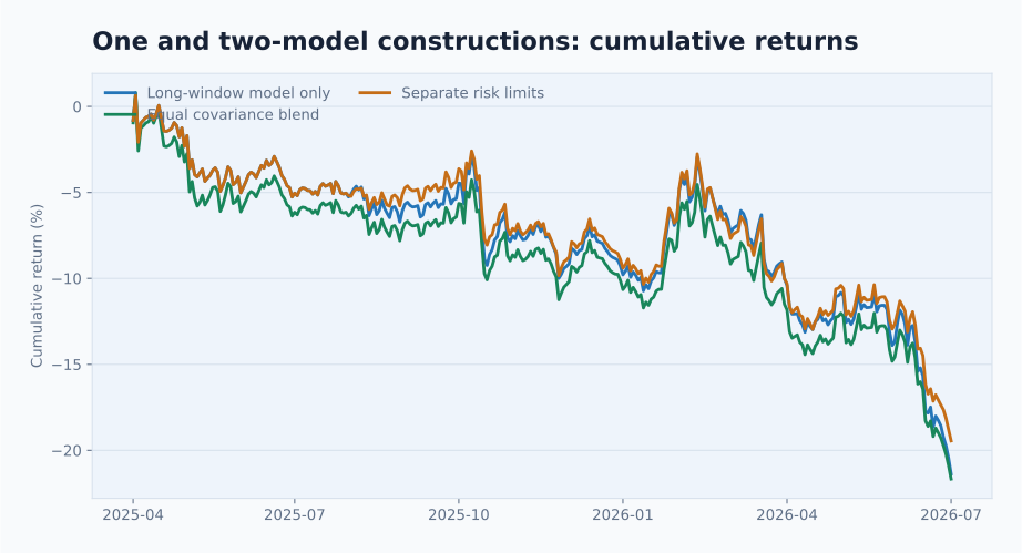
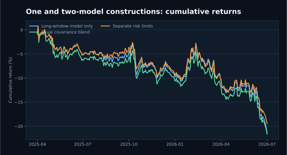
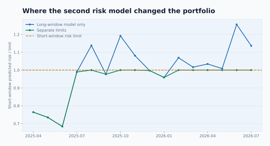
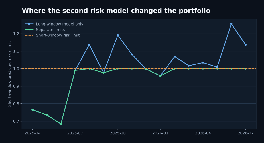
The portfolio constrained only by the longer-history model exceeded the shorter-history model's limit at nine of sixteen reporting rebalances. Enforcing both limits reduced average realized volatility in the nine following intervals from 11.23% to 10.37% annualized. An equal covariance blend exceeded the long-window component limit five times and the short-window component limit eight times while satisfying its own blended limit.
The evidence covers nine breach episodes, and every construction lost money over the full reporting period. It supports the second model as a risk control within this sample, with a larger study needed to assess performance across factor sets and market conditions.
Two estimates of the same portfolio risk
Let \(\Sigma_{L,t}\) be a covariance estimated from the previous 126 observations and \(\Sigma_{S,t}\) one estimated from the previous 42. For factor-allocation weights \(\mathbf w_t\), the two predicted risks are
\[\sigma_{L,t}(\mathbf w_t) = \sqrt{\mathbf w_t^{\mathsf T}\Sigma_{L,t}\mathbf w_t}, \qquad \sigma_{S,t}(\mathbf w_t) = \sqrt{\mathbf w_t^{\mathsf T}\Sigma_{S,t}\mathbf w_t}.\]
The long window changes slowly and estimates covariance from more observations. The short window responds more quickly when factor volatilities and correlations move. Both matrices use 25% shrinkage toward their own diagonals, so the comparison changes the horizon while keeping the estimator family fixed.
At each rebalance, the limit under model \(m\) is 110% of that model's predicted risk for an equal-weight allocation:
\[\tau_{m,t} = 1.10\sqrt{ \mathbf w_{EW}^{\mathsf T} \Sigma_{m,t} \mathbf w_{EW} }, \qquad \mathbf w_{EW}=\frac{1}{N}\mathbf 1.\]
This relative definition updates the scale as the covariance estimate changes, while preserving the same 1.10 multiplier throughout the reporting period.
The three constructions
Every construction receives the same trailing 63-observation expected returns, the same eight factor spreads, and the same allocation constraints. Weights are non-negative, sum to one, and cannot exceed 35% in any factor.
The primary construction maximizes expected return subject to the long-window limit:
\[\max_{\mathbf w_t\in\mathcal W} \mathbf w_t^{\mathsf T}\widehat{\boldsymbol\alpha}_t \quad\text{subject to}\quad \sigma_{L,t}(\mathbf w_t)\le\tau_{L,t}.\]
The blend forms one covariance
\[\overline\Sigma_t = \frac{1}{2}\Sigma_{L,t} +\frac{1}{2}\Sigma_{S,t}\]
and applies a single limit scaled from the equal-weight portfolio under that matrix. The third construction retains both matrices and applies both limits:
\[\sigma_{L,t}(\mathbf w_t)\le\tau_{L,t}, \qquad \sigma_{S,t}(\mathbf w_t)\le\tau_{S,t}.\]
A very small quadratic regularizer resolves numerically equivalent expected-return solutions. It is not intended to act as an additional economic risk budget.
import numpy as np

def predicted_risk(weight, covariance):
    return np.sqrt(weight @ covariance @ weight)

def relative_limit(covariance, multiplier=1.10):
    count = covariance.shape[0]
    equal_weight = np.repeat(1.0 / count, count)
    return multiplier * predicted_risk(equal_weight, covariance)

def risk_ratio(weight, covariance, multiplier=1.10):
    return predicted_risk(weight, covariance) / relative_limit(covariance, multiplier)
A ratio below one has slack, a ratio of one is on the declared limit, and a ratio above one is a breach under that model. The optimizer with separate limits admits only portfolios whose long- and short-window ratios are both at or below one.
A recorded breach made tangible
At the October 2025 rebalance, the primary portfolio's short-window risk ratio was 1.192. It was within its long-window limit but 19.2% above the limit that the short-window covariance assigned to the same weights. The dual-constrained allocation brought the short-window ratio back to one.
The ratio is dimensionless. If the contemporaneous short-window limit had been 10% annualized, for example, the same calculation would read
\[\text{primary predicted risk} =1.192(10\%)=11.92\%,\]
while the dual portfolio could carry at most 10% under that model. This 10% number is only a unit illustration; the study used the date-specific covariance and limit in daily units.
Data and evaluation period
The common factor panel runs from 3 April 2024 through 16 July 2026. Each daily factor return is an equal-weight top-decile minus bottom-decile spread formed from registered signals with a one-trading-day feature lag and the next available return. The eight fixed factors cover momentum, reversal, volatility, intraday price relationships, and a technical composite, with average daily security coverage between roughly 1,310 and 1,342 names.
The allocation was recomputed every 21 common observations. Six early rebalances were kept outside the reporting period; the reported comparison contains 320 daily observations and sixteen rebalances from 7 April 2025 to 16 July 2026. All covariances and forecasts stop before the corresponding allocation date.
The 1.10 multiplier is the declared main setting. Runs at 1.05 and 1.25 test whether the conclusion changes when both risk allowances tighten or widen. Returns are gross of transaction costs, borrow, financing, and market impact.
Full-period results
Walk-forward results, gross of transaction costs
| Construction | Annualized return | Annualized volatility | Maximum drawdown | Mean one-way turnover |
|---|---|---|---|---|
| Long-window model only | -17.25% | 10.93% | 21.89% | 39.95% |
| Equal covariance blend | -17.49% | 10.93% | 22.29% | 40.31% |
| Separate long and short limits | -15.66% | 10.30% | 19.98% | 40.11% |
The dual construction lowered full-period volatility by 0.63 percentage point and maximum drawdown by 1.91 percentage points relative to the primary model. Mean turnover was effectively unchanged: 40.11% against 39.95% per rebalance. Its average one-way weight difference from the primary allocation was 4.95%, so the second model usually altered a minority of the factor allocation rather than replacing it.
Return improved from -17.25% to -15.66% annualized, but the small sample and negative performance do not support an expected-return claim. The study asks whether a second covariance improved risk control, and the more direct evidence comes from the dates on which the models disagreed.
What happened when the second model objected
The long-window portfolio breached the short-window limit at nine of sixteen rebalances, a rate of 56.25%. In those nine non-overlapping holding intervals, its mean realized volatility was 11.23% annualized. The dual portfolio's mean realized volatility over the same intervals was 10.37%, a reduction of 0.86 percentage point.
A paired bootstrap that resamples those nine interval differences gives a 95% descriptive interval from -1.77 to -0.06 percentage points for dual minus primary realized volatility. The interval is useful as a small-sample check, but nine episodes are not enough to claim that the same effect will persist across factor sets or market regimes.
The separate limits were active often enough to matter: the long-window constraint was binding at six of sixteen rebalances and the short-window constraint at ten. The figure shows that the dual portfolio coincides with the primary one while the second model has ample slack, then changes as the short-window ratio approaches or crosses one.
Why the covariance blend did not provide the same limit
Variance under an equal blend is the average of the two modeled variances:
\[\mathbf w^{\mathsf T}\overline\Sigma_t\mathbf w = \frac{1}{2} \mathbf w^{\mathsf T}\Sigma_{L,t}\mathbf w + \frac{1}{2} \mathbf w^{\mathsf T}\Sigma_{S,t}\mathbf w.\]
Low risk under one component can therefore offset high risk under the other. The blended constraint was binding at eleven of sixteen rebalances, yet the chosen portfolio exceeded the comparable long-window limit five times and the short-window limit eight times. Those are not solver failures: the blend constrains the average covariance and makes no promise about either component.
The blend's realized volatility was almost identical to the primary method, and its drawdown was slightly larger. In this test, retaining the disagreement as two constraints was more informative than averaging it away.
Sensitivity to the common risk allowance
Results as the equal-weight risk multiplier changes
| Multiplier | Primary short-model breaches | Primary volatility | Dual volatility | Primary drawdown | Dual drawdown | Breach-interval volatility change |
|---|---|---|---|---|---|---|
| 1.05 | 11 of 16 | 10.47% | 9.78% | 20.71% | 18.69% | -0.72 pp |
| 1.10 | 9 of 16 | 10.93% | 10.30% | 21.89% | 19.98% | -0.86 pp |
| 1.25 | 8 of 16 | 11.94% | 11.57% | 23.33% | 23.74% | -0.59 pp |
The dual construction reduced full-period volatility at all three settings. Its drawdown was smaller at 1.05 and 1.10, but slightly larger at 1.25. The paired interval for the breach-period volatility change excluded zero at 1.05 and 1.10; at 1.25 it ran from -1.24 to +0.04 percentage points. The evidence is therefore weaker once the allowance becomes loose, which is consistent with a secondary constraint having less influence.
Conditions under which the second model helped
Four observations support the result in this sample. The two models differed along an interpretable dimension, recent versus longer covariance history. The primary portfolio crossed the secondary limit often enough to create a useful comparison. Enforcing the limit changed the weights without materially raising turnover. Realized volatility then fell specifically in the intervals following those disagreements, as well as over the full reporting period.
The same test could fail elsewhere. A second estimator that closely tracks the first adds little. A tight limit can lower risk merely by suppressing every forecast, while a loose one can remain inactive. Both models can also miss a new covariance regime at the same time. Binding frequency, weight change, and realized risk after disagreements are therefore more revealing than the number of covariance matrices named in an optimizer.
Common implementation mistakes
Comparing risk numbers with different units
Daily and annualized covariance, local and base-currency returns, or active and total risk cannot share a limit until their conventions agree.
Giving one model incomplete coverage
Every held position needs a covariance treatment under every enforced model. Silently omitting uncovered holdings understates the model's risk.
Assuming a covariance blend enforces its components
An average variance limit controls the average. Test component risks explicitly when either component represents a separate concern.
Declaring success because the second constraint binds
A binding constraint proves only that it changed the feasible set. The evaluation must show what changed in holdings, forecast exposure, turnover, drawdown, and realized risk.
Setting the secondary cap from the reporting results
Choose the model roles and candidate limits before examining the final period. Report a sensitivity range so the reader can see when the conclusion weakens.
Treating a short window as a complete stress model
A 42-observation covariance reacts faster than a 126-observation estimate, but both are backward-looking statistical models. Historical scenarios, fundamental exposures, nonlinear instruments, and liquidity risks require their own treatment.
How the comparison enters portfolio evaluation
A multiple-model portfolio record should preserve each named covariance, predicted risk, limit, slack, and binding indicator at the rebalance date. It should also retain the primary-only candidate so the positions responsible for the difference can be traced. Users can then decide whether the second model expresses a relevant risk view and whether its expected-return cost is acceptable for their mandate.
The study can now be extended beyond two statistical windows. A fundamental model, a principal-component estimate, and historical stress covariance can be added when each has point-in-time coverage for the same holdings. They should enter under their actual definitions; relabeling several nearby sample windows as independent models would overstate the available evidence.
Frequently asked questions
Did the second risk model improve returns?
The dual construction lost less in this reporting period, but the experiment was designed around risk control and contains only sixteen rebalances. Its stronger result is the reduction in realized volatility after the nine dates on which the secondary model rejected the primary allocation.
Why use a long and short covariance instead of two different model types?
They can be estimated from the same point-in-time return panel, so horizon is the principal difference. This makes the first test easier to interpret. Structurally different models are a valuable next step once their coverage and units are aligned.
Does a risk-ratio breach mean the portfolio violated a live mandate?
No. The limit is an experimental setting equal to 110% of contemporaneous equal-weight predicted risk. It is used to compare constructions and is not a client mandate or live portfolio limit.
Why did the separate-limit portfolio sometimes remain below both caps?
Position caps, the budget constraint, expected returns, and both covariance geometries interact. A solution can be determined by another constraint or by the expected-return optimum before either risk boundary is reached.
Would more risk models always improve the result?
No. Each additional model can restrict the feasible portfolio and consume forecast exposure. It is useful when it adds credible information about a risk the existing construction understates.
Next reading
- How Do Multiple Risk Models Enter Portfolio Construction?
- Does Forecast-Error Control Stabilize Portfolios?
- What Is an Eigenportfolio?
Sources
- Luiz Koodi Hotta, Carlos Trucíos, Alexandre Rubesam, and André Alves Portela Santos, “Combining Covariance Forecasts for Large-Dimensional Portfolio Optimization”, 2026 working paper. Provides a recent large-universe comparison of covariance forecasts and combination rules under portfolio constraints.
- Hassan T. Anis and Roy H. Kwon, “End-to-End, Decision-Based, Cardinality-Constrained Portfolio Optimization”, European Journal of Operational Research, 2025. Connects factor covariance estimation to the quality of the resulting portfolio decision.
- Sebastian Ceria, François Margot, Anthony Renshaw, and Anureet Saxena, “Novel Approaches to Portfolio Construction: Multiple Risk Models and Multisolution Generation”, in Optimizing Optimization, 2010. Included as the foundational source for the multi-model experiment developed here.
- Daryl Roxburgh, Katja Scherer, and Tim Matthews, “Optimal Solutions for Optimization in Practice”, in Optimizing Optimization, 2010.
- Fiona Kolbert and Laurence Wormald, “Robust Portfolio Optimization Using Second-Order Cone Programming”, in Optimizing Optimization, 2010.
This walkthrough is for research and educational purposes. It illustrates how strategynet.ai organizes signal evidence into factors and scenarios. It provides no recommendation, investment advice, or instruction to trade any security.
Back to Insights