
What Is a Factor-Mimicking Portfolio?
A factor-mimicking portfolio is a set of holdings constructed to represent a chosen factor while controlling specified common risks. Its return history allows researchers to evaluate the factor's volatility, drawdown, turnover, covariance, and implementation costs.
This article explains how factor scores and risk exposures determine those holdings. A worked example develops the weights, followed by the constraints and trading conventions needed to evaluate the portfolio through time.
Mathematical definition
At time \(t\), let \(\mathbf{x}_t\) contain the normalized exposure of \(N_t\) eligible securities to one factor, \(Q_t\) their point-in-time covariance matrix, and \(B_t\) a matrix of exposures to be controlled. One pure construction is
\[\begin{aligned} \min_{\mathbf{w}_t}\quad & \frac{1}{2}\mathbf{w}_t^\top Q_t\mathbf{w}_t \\ \text{subject to}\quad & \mathbf{w}_t^\top\mathbf{x}_t=1, \\ & \mathbf{w}_t^\top\mathbf{1}=0, \\ & B_t^\top\mathbf{w}_t=\mathbf{0}, \\ & \mathbf{w}_t\in\mathcal{W}_t. \end{aligned}\]
Unit exposure to the selected factor is imposed by \(\mathbf{w}_t^\top\mathbf{x}_t=1\), dollar neutrality by \(\mathbf{w}_t^\top\mathbf{1}=0\), and removal of the declared common exposures by \(B_t^\top\mathbf{w}_t=\mathbf{0}\). The set \(\mathcal{W}_t\) contains position, gross, liquidity, borrowing, and turnover limits. Other constructions use characteristic sorts or proportional scores, but their timing and weighting rules still need to be explicit.
If the weights are fixed at \(t\) and the next-period security returns are \(\mathbf{r}_{t+1}\), the factor portfolio return after implementation cost is
\[r^F_{t+1} = \mathbf{w}_t^\top\mathbf{r}_{t+1}-c_{t+1}.\]
Reconstructing this portfolio at each historical rebalance produces the point-in-time factor return history used in validation.
Four-security worked example
Suppose four securities have factor exposures
\[\mathbf{x} = \begin{bmatrix} 1.0 & 0.5 & -0.5 & -1.0 \end{bmatrix}^{\mathsf T}.\]
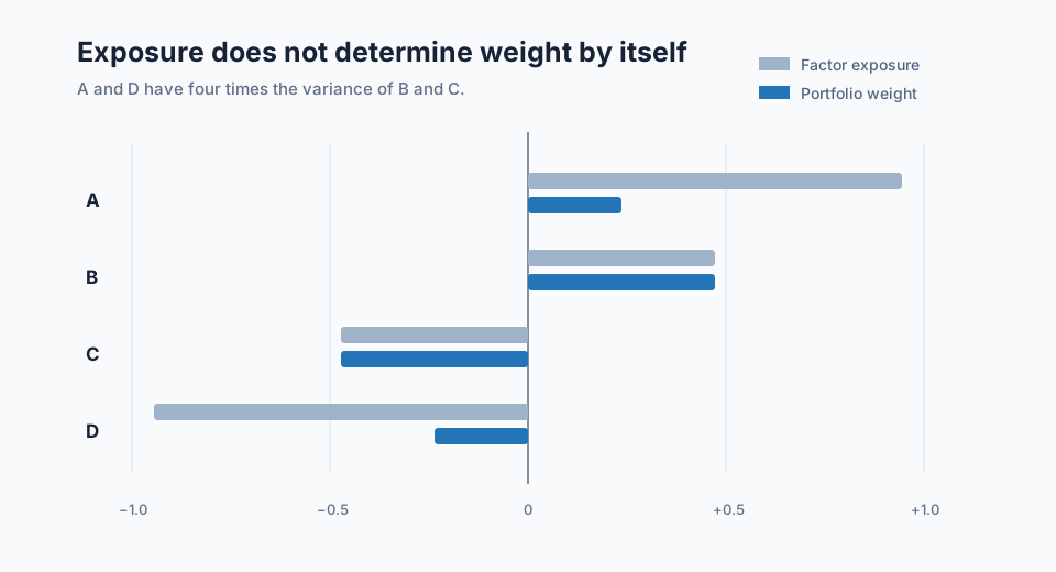
A and D have the strongest scores, but their variances are four times those of B and C. Use the diagonal covariance matrix
\[Q = \operatorname{diag}(4,1,1,4).\]
Symmetry and dollar neutrality imply weights of the form \(\mathbf{w}=(a,b,-b,-a)^{\mathsf T}\). Unit factor exposure requires
\[\mathbf{w}^{\mathsf T}\mathbf{x}=2a+b=1.\]
Portfolio variance is
\[\mathbf{w}^{\mathsf T}Q\mathbf{w}=8a^2+2b^2.\]
Substituting \(b=1-2a\) and minimizing gives \(a=0.25\) and \(b=0.50\):
\[\mathbf{w} = \begin{bmatrix} 0.25 & 0.50 & -0.50 & -0.25 \end{bmatrix}^{\mathsf T}.\]
The lower-risk middle securities receive larger absolute weights even though their factor scores are smaller.
Minimum-risk weights with unit factor exposure
| Security | Factor exposure | Relative variance | Portfolio weight |
|---|---|---|---|
| A | +1.0 | 4 | +25% |
| B | +0.5 | 1 | +50% |
| C | −0.5 | 1 | −50% |
| D | −1.0 | 4 | −25% |
The weights have zero net exposure, 150% gross exposure, and unit exposure to the signal:
\[0.25(1)+0.50(0.5)-0.50(-0.5)-0.25(-1)=1.\]
From weights to a factor return
Suppose next-period returns are \(+3\%\), \(+1\%\), \(-1\%\), and \(-2\%\). Before costs, the factor portfolio earns
\[\begin{aligned} r^F &=0.25(3\%)+0.50(1\%)-0.50(-1\%)-0.25(-2\%)\\ &=2.25\%. \end{aligned}\]
Every position contributes positively in this constructed period because the positive-score securities rise and the negative-score securities fall. One period says nothing about reliability; the same frozen-weight calculation must be repeated across later returns.
Python calculation
import numpy as np

factor_exposure = np.array([1.0, 0.5, -0.5, -1.0])
covariance = np.diag([4.0, 1.0, 1.0, 4.0])

# Constraints: unit factor exposure and zero net weight.
constraints = np.column_stack([factor_exposure, np.ones(4)])
targets = np.array([1.0, 0.0])

inverse_covariance = np.linalg.inv(covariance)
weights = (
    inverse_covariance
    @ constraints
    @ np.linalg.inv(constraints.T @ inverse_covariance @ constraints)
    @ targets
)

next_return = np.array([0.03, 0.01, -0.01, -0.02])
factor_return = weights @ next_return

print(np.round(weights, 2))       # [ 0.25  0.50 -0.50 -0.25]
print(round(factor_return, 4))    # 0.0225
Positive, zero, and negative values
A positive security exposure means the factor definition places the security on its positive side; a negative exposure places it on the opposite side. A zero exposure provides no first-order representation of the factor at that date.
A positive factor portfolio return means the weighted positive side outperformed the weighted negative side after the declared construction and costs. A negative return means the ordering moved against the portfolio. The factor's registered direction determines which sign is favourable.
Sorted portfolios and optimized portfolios
A characteristic-sorted factor portfolio can hold the top quantile and short the bottom quantile, often with equal or value weights inside each side. This method is transparent and useful for research attribution. It may carry broad sector, size, beta, or volatility differences unless the sorts control them.
An optimized factor-mimicking portfolio uses a covariance model and explicit exposure constraints. It can represent the factor more precisely under the chosen model, but its result depends on estimated covariance, numerical stability, and the selected constraints. Comparing the two constructions helps show whether performance comes from the factor ranking or from an incidental portfolio choice.
Common implementation mistakes
Building historical weights from current data
Every rebalance needs the universe, scores, covariance, classifications, and constraints available at that time. Current constituents or revised exposures introduce look-ahead bias.
Calling a score vector a portfolio
Scores do not state gross exposure, risk, covariance, liquidity, or cost. Portfolio weights require a separate construction rule.
Using a singular covariance matrix without controls
Highly related securities and short estimation windows can make covariance inversion unstable. Shrinkage, factor structure, regularization, and position limits help control the solution.
Neutralizing the economic idea
The matrix \(B_t\) should contain unwanted exposures. Including the selected factor itself, or a near duplicate, can leave no feasible way to achieve the target exposure.
Ignoring gross and financing conventions
Dollar neutrality does not limit gross leverage. Report long notional, short notional, gross exposure, collateral, financing, and borrowing cost separately.
Evaluating before costs and availability
Hard-to-borrow names, wide spreads, and rapid score changes can make a strong paper factor impractical. Rebalance timing and executable prices belong in the return history.
How StrategyNet uses factor-mimicking portfolios
StrategyNet retains the signal observations, risk-model inputs, construction settings, and dated weights separately. The factor portfolio can therefore be reconstructed and tested walk forward. Its completed return history supplies expected-return, covariance, drawdown, and turnover evidence for later allocation alongside other validated factor portfolios.
The final client portfolio may combine several factors and apply additional mandate constraints. The factor-mimicking portfolio is the controlled return representation of one factor, rather than a complete recommendation.
Frequently asked questions
Must a factor-mimicking portfolio be dollar neutral?
No. Dollar neutrality is common for isolating a cross-sectional relationship, but long-only, benchmark-relative, futures, and macro constructions use other budget conventions.
Why target unit factor exposure?
It gives factor portfolios a defined exposure scale. Volatility or gross normalization may be applied later for comparison or allocation.
Are Fama–French factors factor-mimicking portfolios?
Their documented long-short constructions use portfolios sorted on size, book-to-market, profitability, investment, and related characteristics to represent factor returns. Their exact formation, weighting, and update rules are specific to those published factors.
Can one factor have several mimicking portfolios?
Yes. Sort-based, proportional, minimum-variance, and constrained versions can represent the same score differently. Each construction needs its own version and return history.
Next reading
- What Is Residual Alpha?
- Factor exposure: security and portfolio sensitivity
- From factor observations to portfolio holdings
Sources
- Wayne E. Ferson, Andrew F. Siegel, and Pisun Xu, “Mimicking Portfolios with Conditioning Information”, NBER Working Paper 11020, 2005; published in Journal of Financial and Quantitative Analysis, 2006.
- Eugene F. Fama and Kenneth R. French, “Common Risk Factors in the Returns on Stocks and Bonds”, Journal of Financial Economics, 1993.
- Kenneth R. French, “Description of Fama/French Factors”.
This walkthrough is for research and educational purposes. It illustrates how strategynet.ai organizes signal evidence into factors and scenarios. It provides no recommendation, investment advice, or instruction to trade any security.
Back to Insights