
What Is Residual Alpha?
Residual alpha is the part of an expected-return forecast left after specified common exposures have been removed. It helps researchers identify securities whose forecasts remain attractive after accounting for drivers such as market beta, sector, size, value, and momentum.
The calculation below projects forecasts onto a set of exposures and uses the remaining component in portfolio research. A four-security example shows how that adjustment changes forecasts, followed by guidance on evaluation and portfolio construction.
Cross-sectional definition
Let \(\boldsymbol{\alpha}_t\) be an \(N_t\times1\) vector of raw expected-return forecasts and \(B_t\) an \(N_t\times K\) matrix of common exposures, including an intercept when appropriate. Under regression weights \(W_t\), estimate
\[\widehat{\boldsymbol{\gamma}}_t = \arg\min_{\boldsymbol{\gamma}} (\boldsymbol{\alpha}_t-B_t\boldsymbol{\gamma})^\top W_t (\boldsymbol{\alpha}_t-B_t\boldsymbol{\gamma}).\]
The fitted common component is
\[\widehat{\boldsymbol{\alpha}}^{\mathrm{common}}_t =B_t\widehat{\boldsymbol{\gamma}}_t,\]
and residual alpha is
\[\boldsymbol{\alpha}^{\perp}_t = \boldsymbol{\alpha}_t -B_t\widehat{\boldsymbol{\gamma}}_t.\]
Under a full-rank weighted least-squares calculation, \(B_t^\top W_t\boldsymbol{\alpha}^{\perp}_t=\mathbf{0}\). The residual alpha is orthogonal to the exposures included in the projection under the selected weights. It can still contain omitted, nonlinear, or incorrectly measured common relationships.
Four-security example
Suppose the raw annual expected returns and standardized size exposures are:
Raw forecast and one common exposure
| Security | Size exposure | Raw expected return |
|---|---|---|
| A | −1.0 | 4.20% |
| B | −0.5 | 3.00% |
| C | +0.5 | 2.50% |
| D | +1.0 | 0.30% |
An equal-weight regression of expected return on an intercept and size gives
\[\widehat\alpha_i^{\mathrm{common}} =2.50\%-1.66\%\times\operatorname{size}_i.\]
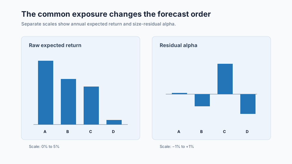
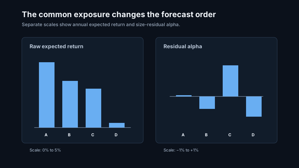
The raw forecast largely favours smaller securities. Subtracting the fitted size component produces:
Common component and residual alpha
| Security | Raw expected return | Size-model estimate | Residual alpha |
|---|---|---|---|
| A | 4.20% | 4.16% | +0.04% |
| B | 3.00% | 3.33% | −0.33% |
| C | 2.50% | 1.67% | +0.83% |
| D | 0.30% | 0.84% | −0.54% |
C has a lower raw forecast than A and B, yet it has the highest residual alpha because its forecast is high relative to what the size relationship predicts. The residuals sum to zero and have zero equal-weight cross-product with size, apart from rounding.
Python calculation
import numpy as np

size_exposure = np.array([-1.0, -0.5, 0.5, 1.0])
raw_expected_return = np.array([0.042, 0.030, 0.025, 0.003])

exposure_matrix = np.column_stack([np.ones(4), size_exposure])
coefficient = np.linalg.lstsq(
    exposure_matrix, raw_expected_return, rcond=None
)[0]

common_component = exposure_matrix @ coefficient
residual_alpha = raw_expected_return - common_component

print(np.round(coefficient, 4))       # [ 0.0250 -0.0166]
print(np.round(residual_alpha, 4))    # [ 0.0004 -0.0033  0.0083 -0.0054]
Residual alpha and realized residual return
A return model observed through time may be written
\[r_{i,t}-r_{f,t} = \alpha_i+\boldsymbol{\beta}_i^\top\mathbf{f}_t+\varepsilon_{i,t}.\]
\(\alpha_i\) is the estimated intercept over the sample, \(\boldsymbol{\beta}_i^\top\mathbf{f}_t\) is the common factor contribution, and \(\varepsilon_{i,t}\) is the realized residual shock at time \(t\). The sample intercept can be called regression alpha, while the residual is the portion of one realized return unexplained by that fitted model.
Cross-sectional residual alpha is a forecast known at the portfolio date. The later realized residual return can be used as its evaluation target. For example, a residual IC compares the ranking of \(\boldsymbol{\alpha}^{\perp}_t\) with the ranking of later returns after the same common exposures have been removed.
Positive, zero, and negative residual alpha
A positive value means the raw forecast lies above the value associated with the included common exposures. A negative value lies below it. Zero means the common-exposure model accounts for the forecast at that observation time.
The sign is conditional on \(B_t\), the regression weights, and the model form. Adding sector or momentum exposure can change both magnitude and order. A positive residual forecast remains uncertain and does not promise a positive realized return.
Residual alpha in portfolio construction
An optimizer can use residual alpha as its expected-return input:
\[\mathbf{w}_t^* = \arg\max_{\mathbf{w}\in\mathcal W_t} \left\{ (\boldsymbol{\alpha}^{\perp}_t)^\top\mathbf{w} -\frac{\lambda}{2}\mathbf{w}^\top Q_t\mathbf{w} -C_t(\mathbf{w}-\mathbf{w}_{t-1}) \right\}.\]
Portfolio constraints can also impose \(B_t^\top\mathbf{w}=0\). Residualizing the forecast changes the expected-return input, while constraining the holdings controls the final portfolio exposure after covariance and implementation effects. The two operations address related parts of the process and can be used together.
Specifying the residualization
The exposure matrix and regression weights determine the common component removed from the forecast. Historical calculations require the classifications and fundamentals available at each observation time. Equal, capitalization, and inverse-variance weights produce different fitted components, with orthogonality defined under the weights used in estimation.
Choose exposures to match the research question. Removing sector effects from a sector-rotation forecast would remove part of the intended relationship. For related exposures such as size and value, a joint projection defines the controlled space consistently; sequential removal can depend on the order.
Interpret the output as an expected residual return under those choices. Realized residuals also contain noise, and zero weighted linear exposure can coexist with nonlinear or regime-dependent relationships. Evaluation should therefore retain the projection settings alongside the forecast and its later outcome.
Signal evaluation
Report raw and residual IC on the same security-date intersection. Their difference shows how much ranking evidence came from common exposures. Also compare quantile spreads, turnover, coverage, stability, and results by group.
A factor-mimicking portfolio built from residual alpha should retain the forecast projection, risk exposures, construction settings, and realized holdings. This makes it possible to determine whether later performance came from security selection, omitted common risk, or constraint choices.
Frequently asked questions
Does residualization make the signal market neutral?
It can remove linear market exposure from the forecast when market beta is included. Final holdings still require an exposure check or constraint.
Can residual alpha be combined with common-factor forecasts?
Yes. Keep the common component and residual component as distinct inputs so their expected returns, risks, and allocations remain attributable.
Should residual alpha be standardized?
Often it is ranked or z-scored after residualization. The transformation changes distance information and should be recorded as part of the factor version.
Next reading
Sources
- Ragnar Frisch and Frederick V. Waugh, “Partial Time Regressions as Compared with Individual Trends”, Econometrica, 1933.
- Eugene F. Fama and Kenneth R. French, “Common Risk Factors in the Returns on Stocks and Bonds”, Journal of Financial Economics, 1993.
- Barr Rosenberg, “Extra-Market Components of Covariance in Security Returns”, Journal of Financial and Quantitative Analysis, 1974.
This walkthrough is for research and educational purposes. It illustrates how strategynet.ai organizes signal evidence into factors and scenarios. It provides no recommendation, investment advice, or instruction to trade any security.
Back to Insights