
Does Forecast-Error Control Stabilize Portfolios?
Forecast-error controls incorporate uncertainty in expected returns into portfolio allocation. This study compares two such controls, a quadratic penalty and an ellipsoidal uncertainty term, to assess their effects on volatility, drawdown, and turnover.
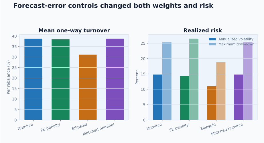
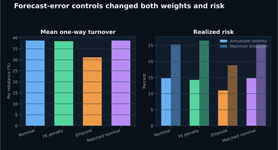
The ellipsoidal term reduced annualized volatility from 14.81% to 11.02%, maximum drawdown from 25.29% to 18.83%, and mean one-way turnover from 38.76% to 31.14% per rebalance. The quadratic penalty produced small changes in allocation and slightly worsened realized return and drawdown.
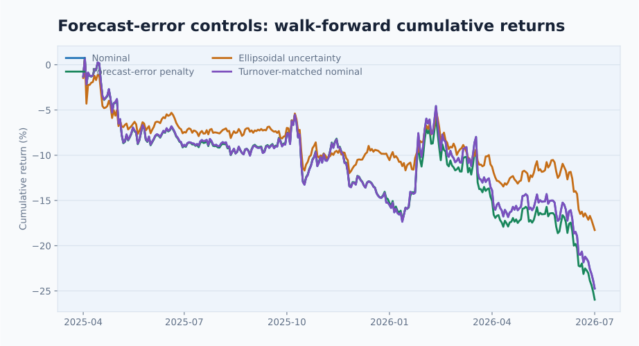
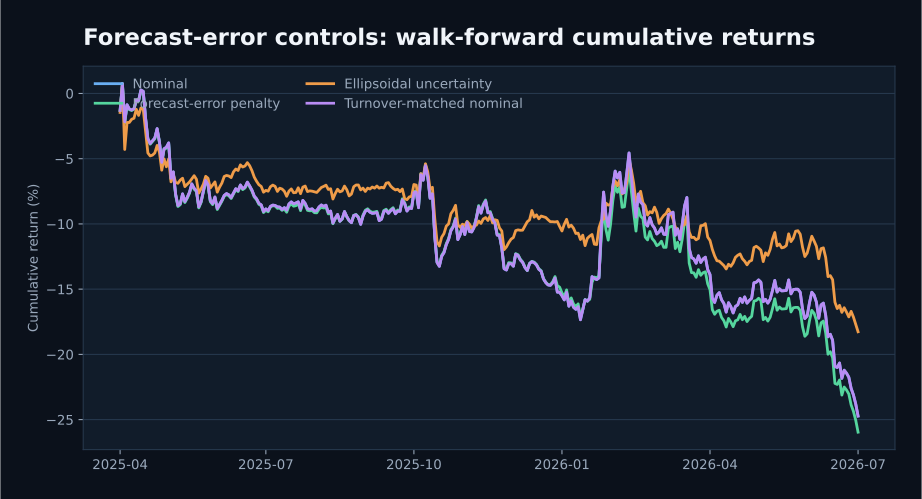
Every construction lost money during the 320-day reporting period, before transaction costs. The results therefore support the ellipsoidal method's use for stability in this sample; its profitability and performance in other periods require further evaluation.
The portfolio and its forecast errors
Let \(\mathbf r_t\) contain the returns of \(N\) factor-spread portfolios on day \(t\). At a rebalance date, the expected-return estimate for factor \(i\) is its trailing 63-observation mean:
\[\widehat{\alpha}_{i,t} = \frac{1}{63}\sum_{s=t-63}^{t-1}r_{i,s}.\]
Once \(r_{i,t}\) is known, the completed one-period forecast error is
\[e_{i,t}=\widehat{\alpha}_{i,t}-r_{i,t}.\]
The sign convention is important. A positive error means the forecast exceeded the realized return; a negative error means the realized return exceeded the forecast. Zero means the forecast and return were equal for that factor and period. The portfolio error is \(\mathbf w_t^{\mathsf T}\mathbf e_t\), so errors that occur together can remain large after several factors have been combined.
The nominal allocation solves
\[\max_{\mathbf w_t\in\mathcal W} \left\{ \mathbf w_t^{\mathsf T}\widehat{\boldsymbol\alpha}_t -\frac{\lambda}{2} \mathbf w_t^{\mathsf T}\Sigma_t\mathbf w_t \right\},\]
where \(\Sigma_t\) is a 126-observation return covariance, \(\lambda=2\), and \(\mathcal W\) requires factor-allocation weights to sum to one, remain non-negative, and stay at or below 35%. Each underlying factor spread is itself a long-short return.
Two ways of carrying the errors into allocation
The first treatment estimates the trailing error mean \(\mathbf m_{e,t}\) and error covariance \(\Omega_{e,t}\) from as many as 126 completed forecasts. It subtracts the error variance and squared bias from the nominal objective:
\[\max_{\mathbf w_t\in\mathcal W} \left\{ \mathbf w_t^{\mathsf T}\widehat{\boldsymbol\alpha}_t -\frac{\lambda}{2}\mathbf w_t^{\mathsf T}\Sigma_t\mathbf w_t -\frac{\eta}{2} \left( \mathbf w_t^{\mathsf T}\Omega_{e,t}\mathbf w_t +(\mathbf m_{e,t}^{\mathsf T}\mathbf w_t)^2 \right) \right\},\]
with \(\eta=1\) in the main run. This discourages combinations whose historical errors were variable or persistently biased, but its quadratic scale can leave the allocation close to the nominal solution.
The second treatment estimates the uncertainty of the forecast mean using a five-lag heteroskedasticity-and-autocorrelation-consistent covariance, \(\Omega_{\widehat\alpha,t}\). It then maximizes the lower value of expected return inside an ellipsoid:
\[\max_{\mathbf w_t\in\mathcal W} \left\{ \mathbf w_t^{\mathsf T}\widehat{\boldsymbol\alpha}_t -k\sqrt{ \mathbf w_t^{\mathsf T} \Omega_{\widehat\alpha,t} \mathbf w_t } -\frac{\lambda}{2}\mathbf w_t^{\mathsf T}\Sigma_t\mathbf w_t \right\}.\]
The main radius is \(k=1.645\). It controls the size of the uncertainty set; it is not presented as an exact 95% probability statement for future returns.
import numpy as np

def nominal_value(weight, alpha, return_cov, risk_aversion=2.0):
    return weight @ alpha - 0.5 * risk_aversion * (weight @ return_cov @ weight)

def error_penalty(weight, error_mean, error_cov, strength=1.0):
    variance = weight @ error_cov @ weight
    squared_bias = (error_mean @ weight) ** 2
    return 0.5 * strength * (variance + squared_bias)

def ellipsoid_penalty(weight, alpha_uncertainty, radius=1.645):
    return radius * np.sqrt(weight @ alpha_uncertainty @ weight)
These functions reproduce the three objective components. The study used a constrained numerical optimizer around them and checked the budget, individual weight cap, and positive-semidefinite covariance conditions at every rebalance.
Data and walk-forward design
The input panel contains eight economically distinct registered factors: five- and 20-day momentum, one-day reversal, low alpha volatility, low realized volatility, the prior-day close/VWAP gap, the prior-day residual open/close move, and a technical-oscillator composite. The list was fixed by factor type and common-history availability, without using reporting-period performance.
For each factor and date, the return is the equal-weight return of the top signal decile minus the equal-weight return of the bottom decile. The registered factor value receives a one-trading-day feature lag and is evaluated against the next available return. Average daily security coverage ranged from about 1,310 to 1,342 names.
Walk-forward specification
| Item | Setting |
|---|---|
| Common panel | 572 dates, 3 April 2024 to 16 July 2026 |
| Forecast | Trailing 63-observation mean |
| Return covariance | Trailing 126 observations, 25% shrinkage toward the diagonal |
| Forecast errors | Up to 126 completed errors; minimum 30 |
| Rebalance interval | 21 common observations |
| Calibration | First 6 rebalances, 2 October 2024 to 7 March 2025 |
| Reporting | 320 days and 16 rebalances, 7 April 2025 to 16 July 2026 |
All estimates stop before the allocation date. The first six rebalances were excluded from reporting and used to choose the nominal risk-aversion value that most closely matched the quadratic method's turnover. The selected value was the original \(\lambda=2\), so the turnover-matched control and nominal portfolio are identical in the reporting period.
Returns in this article are gross factor-spread returns. They do not include transaction costs, borrow, financing, market impact, or the security-level constraints that would be required for an investable portfolio.
Results
Walk-forward results, gross of transaction costs
| Construction | Annualized return | Annualized volatility | Maximum drawdown | Mean one-way turnover | Daily forecast RMSE |
|---|---|---|---|---|---|
| Nominal | -20.04% | 14.81% | 25.29% | 38.76% | 0.961% |
| Quadratic error penalty | -21.08% | 14.28% | 26.51% | 38.45% | 0.931% |
| Ellipsoidal uncertainty | -14.69% | 11.02% | 18.83% | 31.14% | 0.720% |
| Turnover-matched nominal | -20.04% | 14.81% | 25.29% | 38.76% | 0.961% |
The ellipsoidal method reduced volatility by 3.79 percentage points, or 25.6% relative to the nominal portfolio. Its drawdown was 6.46 percentage points smaller and its turnover was 7.62 percentage points lower per rebalance. For a quick check, the relative volatility change is
\[\frac{14.81\%-11.02\%}{14.81\%}=25.6\%.\]
It also accepted less forecast exposure: its average forecast, annualized for comparison, was 22.76%, against 30.13% for the nominal method. The optimizer accepted lower estimated return in exchange for less concentration in forecasts whose uncertainty moved together.
The quadratic error penalty reduced volatility by only 0.52 percentage point and turnover by 0.31 percentage point. It lowered forecast RMSE slightly, yet the annualized return and drawdown were worse. Historical forecast-error variance was therefore too weak a control, at this scale, to change the main allocation problem.
Sensitivity to the uncertainty setting
The main conclusion should not depend on one finely chosen coefficient. The quadratic penalty was rerun at weights of 0.5, 1, and 2; the ellipsoid was rerun at radii of 1, 1.645, and 2.
Sensitivity results
| Method and setting | Annualized return | Volatility | Maximum drawdown | Mean turnover |
|---|---|---|---|---|
| Quadratic η = 0.5 | -20.52% | 14.51% | 25.86% | 38.64% |
| Quadratic η = 1 | -21.08% | 14.28% | 26.51% | 38.45% |
| Quadratic η = 2 | -21.59% | 14.12% | 27.10% | 38.57% |
| Ellipsoid k = 1 | -19.93% | 12.42% | 25.12% | 38.17% |
| Ellipsoid k = 1.645 | -14.69% | 11.02% | 18.83% | 31.14% |
| Ellipsoid k = 2 | -13.88% | 10.62% | 17.85% | 30.27% |
Larger ellipsoids progressively lowered forecast exposure, volatility, drawdown, and turnover. The direction is consistent across the three radii, although the better realized return at larger radii occurred in this particular reporting period and should not be extrapolated. Increasing the quadratic coefficient also lowered volatility, but only slightly, and drawdown continued to worsen.
Why a positive forecast produced a negative return
All four methods carried positive trailing-mean forecasts while recording negative realized returns. The nominal portfolio's average forecast was 30.13% on an annualized scale, yet its annualized realized return was -20.04%. This is exactly the circumstance forecast-error controls are intended to address: an optimizer can be internally consistent while its expected-return input is wrong.
A negative realized portfolio return says that the weighted factor spreads lost money over the interval. It does not prove that every factor definition is invalid, and a less negative result does not establish that an uncertainty model will be profitable elsewhere. The reporting period contains one factor set, one market history, and sixteen allocation decisions.
Common mistakes when testing forecast-error controls
Letting the error estimate see the return it is meant to predict
The error for date \(t\) becomes available only after the matching return is known. Including it in the portfolio formed at \(t\) creates look-ahead bias.
Mixing daily and annual inputs inside the objective
Expected returns, return covariance, and error covariance must share a time unit. Annualization belongs in reporting unless every optimization input is converted consistently.
Treating lower volatility as proof of a better signal
An uncertainty penalty can lower risk by reducing forecast exposure. Report the forecast, concentration, and holdings change alongside realized risk.
Ignoring correlated forecast errors
Several signals may depend on the same prices, horizons, or economic mechanism. A diagonal error covariance gives full diversification credit to errors that often arrive together.
Choosing the coefficient from the final cumulative-return chart
The radius or penalty strength should be declared in a calibration procedure and then evaluated in a later interval. A sensitivity grid helps reveal whether the conclusion exists only at one setting.
Adding costs without a constituent trading model
Factor-spread turnover does not by itself determine commissions, spread costs, borrow, or market impact. This study leaves returns gross until those inputs can be estimated at the traded-security level.
How the result enters portfolio evaluation
Forecast uncertainty is most useful as an additional portfolio record rather than as a replacement for the nominal forecast. Each rebalance can retain the dated forecast, completed-error window, uncertainty covariance, radius, nominal expected return, robust lower value, chosen weights, and both the predicted and realized outcomes. A user can then compare allocations under several uncertainty settings without changing the underlying factor research.
The next experiment should repeat this design across different factor groups and market intervals, then move from factor-spread allocations to constituent holdings. That extension will show whether lower factor-level turnover survives security-level constraints and whether the reduction remains after an agreed transaction-cost model.
Frequently asked questions
Did forecast-error control work in this study?
The ellipsoidal construction materially improved the reported stability and risk measures. The quadratic penalty did not. Neither construction made the factor allocation profitable.
Why estimate uncertainty in the forecast mean with a HAC covariance?
Completed forecast errors can be serially dependent. A heteroskedasticity-and- autocorrelation-consistent estimate carries several lagged error covariances into the uncertainty of the mean instead of assuming every daily error is independent.
Is 1.645 always the correct ellipsoid radius?
No. It is a declared setting in this study. Its probabilistic meaning depends on how the error distribution and uncertainty set are calibrated, so practical work should examine coverage and results across several fixed radii.
Why include a turnover-matched nominal control?
A robust portfolio may look steadier simply because it carries less forecast exposure. Matching nominal turnover in an earlier interval helps test whether an apparent improvement can be explained by general regularization alone. Here the grid selected the original nominal risk aversion, so the control added no separate line of evidence.
Can these returns be interpreted as a live StrategyNet portfolio?
No. They are diagnostic combinations of equal-weight factor-decile spreads. They do not include a client's factors, constraints, security holdings, costs, or execution decisions.
Next reading
- What Is Alpha Uncertainty?
- When Does a Second Risk Model Improve Portfolio Construction?
- Robust Portfolio Optimization
Sources
- Stefano Benati and Eduardo Conde, “A Relative Robust Approach on Expected Returns with Bounded CVaR for Portfolio Selection”, European Journal of Operational Research, 2022. Studies stable portfolio selection when expected returns and economic scenarios are uncertain.
- Man Yiu Tsang, Tony Sit, and Hoi Ying Wong, “Robust Portfolio Optimization with Respect to Spectral Risk Measures Under Correlation Uncertainty”, Applied Mathematics & Optimization, 2022. Treats ambiguity in portfolio correlation through a distributionally robust formulation.
- Daryl Roxburgh, Katja Scherer, and Tim Matthews, “Optimal Solutions for Optimization in Practice”, in Optimizing Optimization, 2010.
- Fiona Kolbert and Laurence Wormald, “Robust Portfolio Optimization Using Second-Order Cone Programming”, in Optimizing Optimization, 2010.
- Whitney K. Newey and Kenneth D. West, “A Simple, Positive Semi-Definite, Heteroskedasticity and Autocorrelation Consistent Covariance Matrix”, Econometrica, 1987. Included for the foundational HAC covariance estimator used in the article's uncertainty calculation.
This walkthrough is for research and educational purposes. It illustrates how strategynet.ai organizes signal evidence into factors and scenarios. It provides no recommendation, investment advice, or instruction to trade any security.
Back to Insights