What Is Factor Breadth?

Factor breadth is the number of independent investment decisions made over a stated period. A daily cross-sectional factor applied to hundreds of securities does not automatically have hundreds of independent decisions: securities share industries and macroeconomic risks, scores can be correlated, forecast horizons can overlap, and repeated rebalances may express nearly the same view.

Breadth matters because modest forecast skill can become economically useful when it is applied repeatedly to sufficiently independent opportunities. It is therefore a property of the decision process and its dependence structure, not a synonym for universe size.

Definition under independent decisions

In the Fundamental Law of Active Management, breadth \(BR\) is the count of independent forecasts over the measurement period. Under equal skill and an ideal unconstrained implementation, expected Information Ratio is approximated by

\[IR\approx IC\sqrt{BR},\]

where \(IC\) is forecast-return correlation. The square root matters: quadrupling independent breadth doubles the potential Information Ratio under the law's assumptions.

The period must be stated. A breadth estimate of 100 per year and a breadth estimate of 100 per month describe different opportunity rates. Forecast and return horizons also need compatible timing.

Effective breadth with correlated decisions

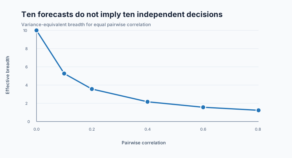
Suppose \(N\) equal-sized decisions have a common pairwise correlation \(\rho\). The variance-equivalent number of independent decisions is

\[BR_{\mathrm{eff}} = \frac{N}{1+(N-1)\rho}.\]

This follows by comparing the variance of the average correlated decision with the variance of an average formed from independent decisions. More generally, if \(C\) is the correlation matrix and the decisions receive equal unit importance,

\[BR_{\mathrm{eff}} = \frac{N^2}{\mathbf{1}^\top C\mathbf{1}}.\]

This is one practical dependence adjustment for an equal-decision example. It is not a universal breadth estimator for every portfolio. Unequal sizing, changing correlations, nonlinear dependence, and overlapping holding periods require a model consistent with the actual decisions.

Ten-decision example

If ten forecasts were independent, breadth would be 10. With average pairwise correlation \(0.20\),

\[BR_{\mathrm{eff}} = \frac{10}{1+9(0.20)} =3.57.\]

At an IC of \(0.05\), the independent-bet approximation gives

\[IR_{\rho=0}=0.05\sqrt{10}=0.158,\]

while the correlation-adjusted approximation gives

\[IR_{\rho=0.20}=0.05\sqrt{3.57}=0.094.\]

The forecast skill is unchanged. Dependence reduces the amount of distinct information applied by the portfolio.

Python calculation

import numpy as np

decision_count = 10
pairwise_correlation = np.array([0.00, 0.10, 0.20, 0.40, 0.60, 0.80])

effective_breadth = decision_count / (
    1 + (decision_count - 1) * pairwise_correlation
)

information_coefficient = 0.05
potential_information_ratio = (
    information_coefficient * np.sqrt(effective_breadth)
)

print(np.round(effective_breadth, 2))
# [10.00  5.26  3.57  2.17  1.56  1.22]

Cross-sectional and time-series breadth

Cross-sectional breadth comes from contemporaneous decisions across securities, countries, contracts, or markets. Time-series breadth comes from decisions made at different observation times. Both can be overstated.

Stocks in one industry may share one dominant earnings or macroeconomic shock. A daily signal with a 20-day holding period produces overlapping positions, so twenty daily rebalances do not create twenty independent time decisions. A global strategy can also repeat the same dollar, rate, or volatility exposure through several instruments.

Breadth analysis should therefore examine score correlation, realized factor portfolio correlation, common exposure, holding-period overlap, and decision turnover. The relevant dependence is the dependence of the implemented bets, rather than the number of rows emitted by a calculation.

Breadth, diversification, and coverage

Coverage is the share of the eligible universe with a valid score. Wider coverage can create more potential decisions, but those decisions may remain highly related. Diversification measures how portfolio risk is distributed, while breadth counts independent opportunities under a forecast process. The concepts are connected and not identical.

A portfolio can hold many securities and have low factor breadth because every holding expresses one macroeconomic view. Another portfolio can use a small set of futures across unrelated markets and have greater effective breadth.

Interpreting breadth values

Breadth is non-negative. A value near one means the decision set behaves roughly like one independent opportunity under the selected estimator. Larger values indicate more distinct decisions. Zero means no active decision was available or the estimator has become degenerate; negative breadth has no interpretation under the standard definition.

Estimated breadth can exceed a raw count when decisions are negatively related. That result should be inspected carefully because correlations are noisy and can change during stress. It should not be treated as unlimited opportunity.

Common implementation mistakes

Using security count as breadth

One thousand securities exposed to the same factor shock do not constitute one thousand independent bets.

Multiplying daily decisions by trading days

Overlapping horizons, persistent scores, and slow portfolio turnover reduce time-series independence.

Estimating dependence on the full history

Live breadth estimates and historical simulations need correlations estimated from information available before each decision date.

Treating small correlations as harmless

With many decisions, modest positive correlation materially reduces effective breadth because it appears in \(1+(N-1)\rho\).

Ignoring factor portfolios

Raw score correlations can differ from correlations after covariance, neutralization, and constraints. Inspect the implemented factor returns as well as the source signals.

Adding breadth across unrelated measurement periods

Breadth per rebalance, month, and year cannot be added until their timing and overlap conventions have been reconciled.

Role in portfolio evaluation

Breadth explains why a low-IC factor can still support a useful portfolio when the signal is applied across many independent opportunities. It also explains why an apparently large research universe can disappoint when its bets share the same exposures.

Strategy evaluation should report the raw opportunity count, an explicit dependence adjustment, score and factor-return correlations, turnover, coverage, and the period over which breadth is measured. The generalized Fundamental Law also includes the transfer coefficient, which measures how much forecast information survives portfolio constraints.

Frequently asked questions

Is breadth the number of holdings?

No. Holdings are implementation outputs. Breadth concerns independent active decisions and can be much smaller than the holding count.

Can two signals on the same stock add breadth?

They can if they supply distinct forecast information and create sufficiently independent implemented decisions. Two transformations of the same underlying input usually add little.

Does a faster rebalance always increase breadth?

No. If the forecast and positions persist, more frequent calculation repeats the same information and increases turnover without adding independence.

How should breadth be estimated in practice?

Start from the actual decision units, state the measurement period, and measure dependence using point-in-time signal, exposure, and factor-return records. Compare several reasonable estimators because effective breadth is model dependent.

Next reading

• What Is the Transfer Coefficient?
• What Is the Fundamental Law of Active Management?
• When Is an Information Coefficient Reliable?

Sources

• Richard C. Grinold, “The Fundamental Law of Active Management”, The Journal of Portfolio Management, 1989.
• Roger G. Clarke, Harindra de Silva, and Steven Thorley, “Portfolio Constraints and the Fundamental Law of Active Management”, Financial Analysts Journal, 2002.