strategynet.ai — Insights

Covariance Shrinkage in Factor Risk Models · Published 2026-07-20

2026-07-20GlossaryDeep dive

Covariance Shrinkage in Factor Risk Models

Covariance shrinkage combines an estimated covariance matrix with a more stable target. The estimate may respond quickly to recent changes while carrying substantial sampling error; the target usually changes more slowly, imposes useful structure, or draws on a longer history. Their combination can improve conditioning and reduce the tendency of an optimizer to make large allocations from small estimated covariance differences.

The method does not make a covariance forecast reliable merely by moving it toward another matrix. The target must represent a plausible source of information, both matrices must describe the same assets and units, and the shrinkage weight must be selected without using the returns it is later asked to predict.

Definition

Let \(\widehat\Sigma_t\) be a responsive covariance estimate available at time \(t\), and let \(T_t\) be a stable target. Linear shrinkage forms

\[\Sigma_{\lambda,t} = (1-\lambda)\widehat\Sigma_t + \lambda T_t, \qquad 0\leq\lambda\leq1.\]

At \(\lambda=0\), the responsive estimate is retained. At \(\lambda=1\), the target is used throughout. Values between those endpoints exchange some responsiveness for stability. A target might be the diagonal of the responsive estimate, a constant-correlation matrix, a long-history covariance, a fundamental risk model, or another independently specified forecast.

If both inputs are positive semidefinite, every convex combination is also positive semidefinite because, for any portfolio \(w\),

\[w^{\mathsf T}\Sigma_{\lambda,t}w = (1-\lambda)w^{\mathsf T}\widehat\Sigma_tw + \lambda w^{\mathsf T}T_tw \geq0.\]

The portfolio variance is a weighted average of the two variance forecasts. Volatility is obtained after that average:

\[\sigma_{\lambda}(w) = \sqrt{ (1-\lambda)\sigma_{\widehat\Sigma}^2(w) + \lambda\sigma_T^2(w) }.\]

Averaging the two volatility numbers directly gives a different result.

A two-asset calculation

Suppose a responsive model and a slower target estimate annual covariance for two assets as

\[\widehat\Sigma = \begin{bmatrix} 0.0400 & 0.0240\\ 0.0240 & 0.0900 \end{bmatrix}, \qquad T = \begin{bmatrix} 0.0225 & 0.0090\\ 0.0090 & 0.0400 \end{bmatrix}.\]

The responsive model assigns volatilities of 20% and 30% with correlation 0.40. The target assigns 15% and 20% with correlation 0.30. Shrinking the responsive estimate 25% toward the target gives

\[\Sigma_{0.25} =0.75\widehat\Sigma+0.25T = \begin{bmatrix} 0.035625 & 0.020250\\ 0.020250 & 0.077500 \end{bmatrix}.\]

For weights \(w=(0.60,0.40)^{\mathsf T}\), the responsive model forecasts variance of 0.04032 and the target forecasts 0.01882. The shrunk forecast is

\[0.75(0.04032)+0.25(0.01882)=0.034945,\]

which corresponds to annualized volatility of approximately 18.69%. The direct weighted average of the two model volatilities would be approximately 18.49%, so it would not preserve the covariance calculation.

import numpy as np

responsive = np.array([
    [0.0400, 0.0240],
    [0.0240, 0.0900],
])
target = np.array([
    [0.0225, 0.0090],
    [0.0090, 0.0400],
])
weight = np.array([0.60, 0.40])
shrinkage = 0.25

combined = (1 - shrinkage) * responsive + shrinkage * target
variance = weight @ combined @ weight
volatility = np.sqrt(variance)

print(combined)
print(f"variance: {variance:.6f}")
print(f"volatility: {volatility:.2%}")

The output is the displayed covariance matrix, variance 0.034945, and volatility 18.69%.

Where shrinkage enters a factor model

A factor risk model represents asset covariance as

\[\Sigma=BF B^{\mathsf T}+D,\]

where \(B\) contains asset exposures, \(F\) is the factor-return covariance, and \(D\) contains specific-return covariance, commonly restricted to a diagonal matrix. Shrinkage can be applied after each complete asset covariance has been constructed:

\[\Sigma_{\lambda} = (1-\lambda) (B_1F_1B_1^{\mathsf T}+D_1) + \lambda (B_2F_2B_2^{\mathsf T}+D_2).\]

This is the safest form when the models use different factor definitions, exposure methodologies, or estimation procedures, provided they cover the same ordered asset universe.

When both models genuinely share the same exposure matrix \(B\), their components can instead receive separate shrinkage weights:

\[F^*=(1-\lambda_F)F_1+\lambda_FF_2, \qquad D^*=(1-\lambda_D)D_1+\lambda_DD_2,\]

followed by \(\Sigma^*=BF^*B^{\mathsf T}+D^*\). Separate weights are useful because factor correlations and specific variances need not carry the same estimation error. Component shrinkage becomes misleading when similarly named factors encode different portfolios or normalizations; in that setting, the factor covariance matrices do not share a basis and should not be averaged directly.

Choosing the shrinkage weight

A convenient weight is not necessarily a defensible weight. The selection should be made in a rolling evaluation whose estimate at date \(t\) uses only information available before \(t\). Candidate matrices can be scored against the next return vector using Gaussian negative log likelihood,

\[L_t(\Sigma) = \log|\Sigma| + r_t^{\mathsf T}\Sigma^{-1}r_t,\]

although this score can be sensitive to heavy tails and poorly conditioned eigenvalues. A Student-\(t\) score, eigenvalue floors, and representative- portfolio risk errors provide useful checks. The economic evaluation should also measure realized volatility, drawdown, turnover, concentration, and the activity of the constraints that matter to the intended portfolio.

The estimated weight can be regularized toward a long-run value or penalized for changing too rapidly. This prevents a few unusual observations from moving the combination from one endpoint to the other, thereby turning risk-model selection into an additional source of turnover.

A seeded horizon experiment

The following simulation generates 1,900 daily observations for twelve assets driven by three factors whose volatilities and correlations move between calmer and stressed settings. Every 21 observations, a long-only minimum-variance portfolio is estimated from a blend of 42- and 252-observation covariances. Both input matrices receive 25% diagonal shrinkage, and no asset may exceed 35%.

This is a numerical illustration rather than evidence about a StrategyNet factor or a live investment universe. Its purpose is to make the stability trade-off visible under known, reproducible conditions.

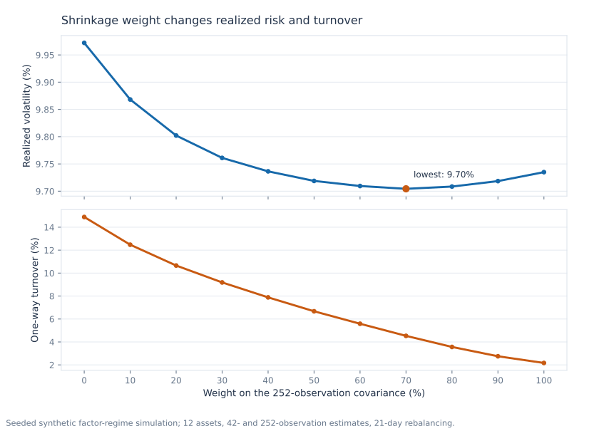
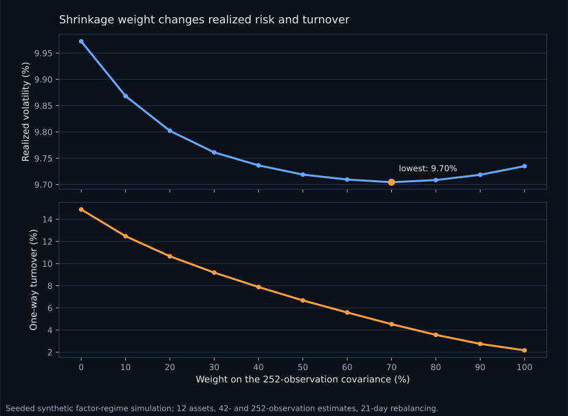
Two line charts vary the weight on a 252-observation covariance from zero to one hundred percent. Realized volatility falls from about 9.97 percent to a minimum near 9.70 percent at seventy percent long-window weight, while one-way turnover falls steadily from about 14.89 percent to 2.17 percent. — In this seeded simulation, the interior blend produced the lowest realized volatility, while greater reliance on the stable target reduced turnover throughout.

The minimum realized volatility occurred with 70% on the long-window estimate and 30% on the short-window estimate: 9.70% annualized, against 9.97% for the short model and 9.73% for the long model. The difference between the interior blend and the long model was small. Turnover moved much more: mean one-way turnover fell from 14.89% under the short estimate to 4.53% at the volatility- minimizing blend and 2.17% under the long estimate.

Those results illustrate why a chosen loss matters. Selecting solely on realized volatility would favour the interior value in this path; including a material turnover penalty could support a heavier long-window weight. The complete runner and aggregate output are stored in run_covariance_shrinkage_simulation.py and its aggregate result record.

Common implementation errors

The estimate and target must have the same asset order, currency, return frequency, forecast horizon, annualization, and missing-observation convention. A covariance measured in daily return units cannot be combined directly with an annualized model, nor can a USD model be treated as interchangeable with an unhedged multi-currency covariance.

Missing cross-covariances should not be filled with zero merely because one model lacks an asset. With partially overlapping universes, the common symbols can support a transfer calibration and validation exercise. With disjoint universes, local covariance matrices do not identify the cross-block covariance; shared factors, synchronized returns, or defensible proxies are required.

The target can also be wrong. A long-history covariance may lag a structural change, while a fundamental model can miss a fast statistical relationship. Shrinkage lowers estimation variance at the cost of bias toward that target, and increasing \(\lambda\) is beneficial only while the variance reduction is worth the added bias.

Finally, an optimizer evaluates particular directions in the covariance matrix rather than an average matrix element. Frobenius error and portfolio-risk error can therefore rank the same candidates differently, especially when the portfolio is concentrated, constrained, leveraged, or designed to neutralize several factors.

Relationship to other combinations

Linear shrinkage is one member of a larger set of covariance combinations. Multiple-target methods use several structured matrices; nonlinear shrinkage regularizes individual eigenvalues; predictive stacking chooses combinations using out-of-sample scores; precision pooling averages inverse covariances; and geometric methods average matrices on the positive-definite cone. These methods answer different questions and should be compared through the decision the risk model is intended to support.

Questions practitioners ask

Is more shrinkage always safer?

No. It usually improves conditioning and can reduce estimation variance, but it also moves the estimate toward the target. A stale or structurally unsuitable target can understate the risk that the responsive model detects.

Can the weight change through time?

Yes, provided it is estimated from completed observations and its instability is controlled. A rapidly changing weight can chase recent forecast errors and produce avoidable turnover.

Should factor covariance and specific risk use the same weight?

Not necessarily. Their sampling error, persistence, and targets differ. Separate weights are coherent when the component definitions align and the resulting asset covariance is checked for symmetry, positive semidefiniteness, variance floors, and conditioning.

What if the models cover different symbols?

A simple covariance average is no longer defined over the missing rows and columns. Partial overlap permits a held-out transfer test; disjoint coverage requires a shared factor or return bridge before cross-universe risk can be estimated.