
What Is the Transfer Coefficient?
The transfer coefficient measures how closely a portfolio's active positions align with its risk-adjusted forecasts. Portfolio managers use it to assess how constraints, such as sector limits or long-only rules, affect the expression of a forecast in the final holdings.
This article defines the coefficient and calculates it for a sector-neutral portfolio. The example connects forecast alignment to the Fundamental Law of Active Management and shows how to assess alignment alongside the risks a constraint controls.
Mathematical definition
Let \(\widetilde{\boldsymbol{\alpha}}_t\) be the vector of risk-adjusted active return forecasts and \(\widetilde{\mathbf{w}}_t\) the corresponding risk-adjusted active positions. The ex ante transfer coefficient is
\[TC_t = \operatorname{corr} \left( \widetilde{\boldsymbol{\alpha}}_t, \widetilde{\mathbf{w}}_t \right).\]
The risk adjustment places forecasts and positions in compatible units under the selected risk model. In an equal-risk example with centred forecasts and positions, the calculation reduces to the ordinary cross-sectional correlation
\[TC = \frac{\boldsymbol{\alpha}^{\mathsf T}\mathbf{w}} {\sqrt{\boldsymbol{\alpha}^{\mathsf T}\boldsymbol{\alpha}} \sqrt{\mathbf{w}^{\mathsf T}\mathbf{w}}}.\]
The risk model, benchmark, forecast centring, and active-weight convention must be stated. Correlating raw forecasts with raw holdings can give a misleading value when securities have materially different risks.
Sector-neutral worked example
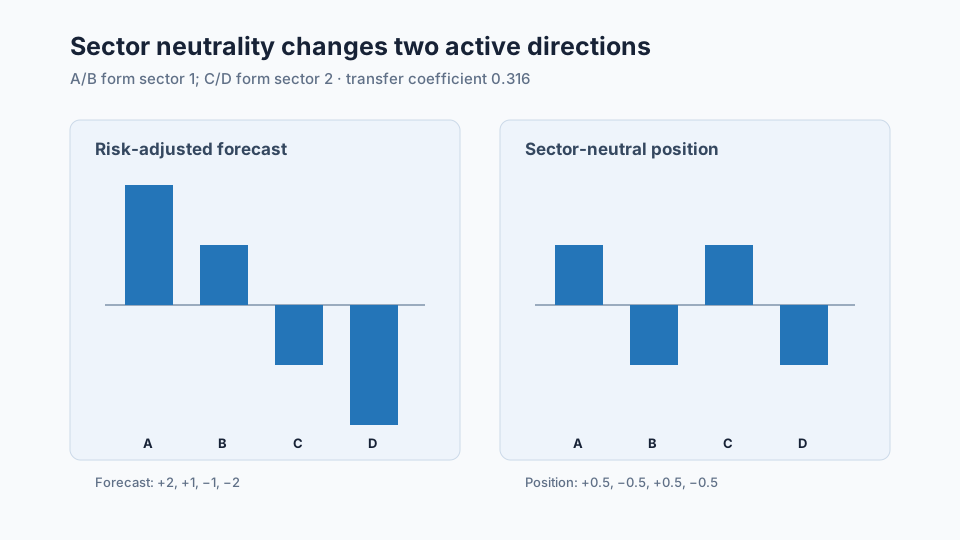
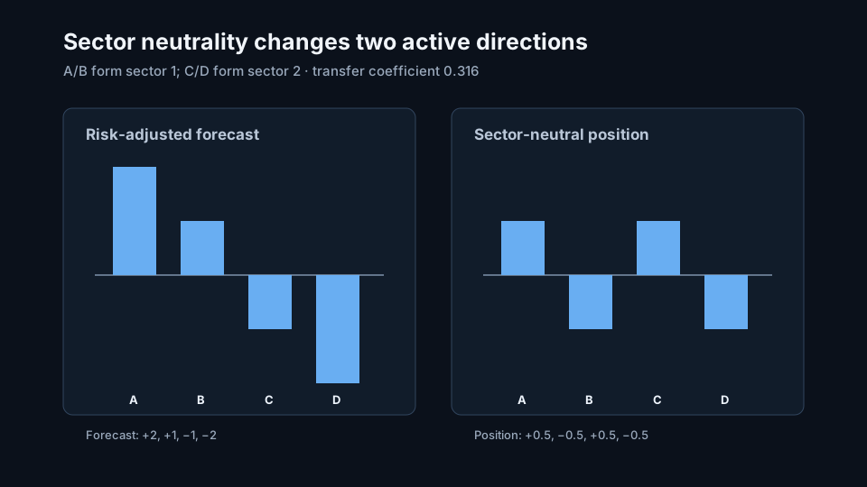
Suppose four equal-risk securities have centred forecasts
\[\boldsymbol{\alpha} = \begin{bmatrix} 2 & 1 & -1 & -2 \end{bmatrix}^{\mathsf T}.\]
A and B belong to sector 1; C and D belong to sector 2. An unconstrained active portfolio would choose positions proportional to the forecasts and have \(TC=1\).
Now impose zero net weight inside each sector. Removing each sector's mean from the forecast gives constrained positions proportional to
\[\mathbf{w} = \begin{bmatrix} 0.5 & -0.5 & 0.5 & -0.5 \end{bmatrix}^{\mathsf T}.\]
The first sector has positive forecasts for both securities, but the constraint requires one long and one short. The same occurs in the negative-forecast sector. The transfer coefficient is
\[TC = \frac{2(0.5)+1(-0.5)+(-1)(0.5)+(-2)(-0.5)} {\sqrt{2^2+1^2+(-1)^2+(-2)^2} \sqrt{4(0.5^2)}} = \frac{1}{\sqrt{10}} =0.316.\]
Forecast transfer before and after sector neutrality
| Security | Sector | Forecast | Unconstrained direction | Sector-neutral position |
|---|---|---|---|---|
| A | 1 | +2.0 | Long | +0.5 |
| B | 1 | +1.0 | Long | −0.5 |
| C | 2 | −1.0 | Short | +0.5 |
| D | 2 | −2.0 | Short | −0.5 |
The constraint removes each sector-level view and retains only the ordering within the sectors. Whether that is desirable depends on whether the research claim concerns sector rotation or security selection within sectors.
Python calculation
import numpy as np

risk_adjusted_forecast = np.array([2.0, 1.0, -1.0, -2.0])
sector_neutral_position = np.array([0.5, -0.5, 0.5, -0.5])

transfer_coefficient = np.corrcoef(
    risk_adjusted_forecast,
    sector_neutral_position,
)[0, 1]

print(round(transfer_coefficient, 3))  # 0.316
The generalized Fundamental Law
The original Fundamental Law relates expected Information Ratio to information coefficient and breadth. A common generalized form includes transfer:
\[IR\approx IC\times TC\times\sqrt{BR}.\]
\(IC\) measures forecast skill, \(BR\) measures independent decisions, and \(TC\) measures how strongly portfolio construction carries those forecasts into positions. If \(IC=0.06\), effective breadth is 100, and \(TC=0.50\), then
\[IR\approx0.06\times0.50\times\sqrt{100}=0.30.\]
The same forecast process with \(TC=0.80\) has a potential Information Ratio of \(0.48\) under the law's assumptions. This calculation is a strategic approximation, not a backtest result.
Ex ante and ex post transfer
Ex ante transfer uses forecasts and proposed holdings known at the portfolio date. It measures the alignment designed into the portfolio. Ex post analysis uses realized returns and performance to study how forecast success and constraint-induced deviations contributed to the outcome.
The two should retain distinct names and dates. A portfolio can have a high ex ante transfer coefficient and poor realized returns because the forecast fails. A low-transfer portfolio can perform well because the constraint-induced positions happen to benefit.
Interpreting positive, zero, and negative values
A positive value means positions generally align with forecasts. One represents perfect positive linear alignment under the chosen risk coordinates. A value near zero means the active positions transmit little of the forecast ordering. A negative value means the implemented positions tend to oppose it.
Transfer is a correlation, so multiplying every position by a positive constant does not change it. It measures alignment rather than aggressiveness. Active risk or tracking error supplies the scale of the portfolio.
Common implementation mistakes
Correlating forecasts with total holdings
Transfer concerns active positions relative to a benchmark or neutral starting point. Benchmark holdings can dominate total weights without representing the forecast.
Ignoring risk adjustment
One dollar in a low-volatility security and one dollar in a high-volatility security do not carry equal risk. The calculation should use coordinates consistent with the portfolio risk model.
Treating low transfer as proof of poor construction
Constraints can serve essential economic and fiduciary purposes. Report both the lost forecast alignment and the risk, cost, or mandate benefit.
Mixing ex ante and realized quantities
Current forecasts paired with later holdings or realized returns do not define an ex ante transfer coefficient. Align every input to the same decision time.
Maximizing transfer in isolation
A portfolio that tracks forecasts perfectly may be concentrated, illiquid, expensive, or exposed to uncontrolled factors. Transfer is one construction diagnostic.
Comparing coefficients from different risk models
Changing covariance, benchmark, or exposure definitions changes the risk-adjusted coordinates. Comparisons require compatible conventions.
Use in portfolio design
Compute the transfer coefficient before and after each important constraint. The sequence can show, for example, that sector neutrality has a small effect, while a turnover limit or long-only boundary removes much of the forecast. This helps decide whether to refine the signal, change the constraint, expand the eligible instruments, or accept the trade-off.
Strategy evaluation should retain IC, effective breadth, transfer coefficient, active risk, expected cost, and the actual exposure limits. These quantities explain different parts of the forecast-to-portfolio mapping.
Frequently asked questions
Is transfer coefficient the same as information coefficient?
No. IC compares forecasts with later returns. TC compares forecasts with the positions produced from them under constraints.
Does scaling the portfolio increase transfer?
No. Positive scaling leaves a correlation unchanged. It increases active risk and expected active return together under a linear model.
Can loosening a constraint reduce transfer?
It can if another binding constraint, interaction, or changed risk model alters the solution. Measure the complete optimization rather than assuming each constraint acts independently.
What transfer coefficient should a portfolio target?
There is no universal threshold. The appropriate value depends on forecast structure, mandate, risk control, costs, available instruments, and the purpose of each constraint.
Next reading
- What Is Factor Breadth?
- What Is the Fundamental Law of Active Management?
- What Is Factor Neutralization?
Sources
- Roger G. Clarke, Harindra de Silva, and Steven Thorley, “Portfolio Constraints and the Fundamental Law of Active Management”, Financial Analysts Journal, 2002.
- Richard C. Grinold, “The Fundamental Law of Active Management”, The Journal of Portfolio Management, 1989.
This walkthrough is for research and educational purposes. It illustrates how strategynet.ai organizes signal evidence into factors and scenarios. It provides no recommendation, investment advice, or instruction to trade any security.
Back to Insights