
How Should Missing Factor Values Be Handled?
Missing factor values affect which securities can be ranked and how their scores should be interpreted. A delayed earnings report, a ratio that does not apply to a bank, and a failed data feed each require a policy suited to the reason the value is absent. Those policies become part of the signal's research definition.
This article examines ways to exclude, replace, or flag missing observations and shows how each choice changes a cross-sectional ranking. Recording the policy and coverage alongside each score makes historical tests reproducible and helps readers judge the evidence available for the current calculation.
Five policies and what each one assumes
Five policies are in common use. They differ less in arithmetic than in what each one assumes about the security whose value is absent, so that assumption is the useful thing to compare them on.
Missing-value policies, by the assumption each one makes
| Policy | What it assumes | Typical use | Main cost |
|---|---|---|---|
| Exclude the observation | The factor has no meaning without the input | Required inputs; sparse gaps | Shrinks the evaluated universe, and rarely at random |
| Neutral normalized component | Absence supplies no directional evidence | Multi-input composites on a normalized scale | Pulls scores toward the centre and hides how thin a score is |
| Peer-group imputation | The security resembles its point-in-time peers | Slow-moving fundamentals with dense peer groups | Imports group bias, creates ties, needs look-ahead controls |
| Carry the last valid observation | The prior value is still economically in force | Scheduled data such as quarterly filings | Goes stale exactly when conditions change; needs a maximum age |
| Renormalize available weights | The observed inputs are a fair sample of the model | Composites where score scale must stay comparable | Each security is then scored by a different effective model |
Coverage and the availability indicator
For input \(k\), define the availability indicator
\[a^{(k)}_{i,t} = \begin{cases} 1, & \text{if a valid point-in-time value is available},\\ 0, & \text{otherwise}. \end{cases}\]
Input coverage at date \(t\) is
\[\operatorname{coverage}^{(k)}_t = \frac{\sum_{i\in U_t}a^{(k)}_{i,t}}{|U_t|}.\]
For a \(K\)-input complete-case composite, security \(i\) is valid only when
\[A_{i,t}=\prod_{k=1}^{K}a^{(k)}_{i,t}=1.\]
This rule preserves a constant definition across securities. In the four-security example below, each of the three inputs is available for three of them, so every input coverage is \(0.75\); only security C carries all three, so complete-case coverage is \(0.25\). Inputs that each look well covered can leave a composite scoring a quarter of the universe, and the shortfall concentrates in whatever the data source covers worst.
What each policy does to the score
Exclude the observation
Exclusion is appropriate when the factor cannot be interpreted without the input. The security remains in the broader investment universe but receives no score from that factor on the date.
Assign neutral normalized exposure
After the observed values have been normalized, set the unavailable component to zero:
\[\widetilde{z}^{(k)}_{i,t} = \begin{cases} z^{(k)}_{i,t}, & a^{(k)}_{i,t}=1,\\ 0, & a^{(k)}_{i,t}=0. \end{cases}\]
This says the missing component supplies no positive or negative evidence. It does not assert that the raw value itself was zero.
Impute from a peer group
A raw value can be replaced by a point-in-time sector, industry, country, or other peer statistic:
\[\widetilde{x}^{(k)}_{i,t} = \operatorname{median} \left\{x^{(k)}_{j,t}:j\in G(i,t),\ a^{(k)}_{j,t}=1\right\}.\]
The group must contain enough valid peers, and the imputed status should remain available downstream. Median imputation reduces extremes and can create many ties.
Carry the last valid observation
Where a value remains economically in force until a scheduled replacement, the observation at \(t\) is the most recent one published by \(t\), subject to a maximum age \(\Delta\):
\[\widetilde{x}^{(k)}_{i,t} = x^{(k)}_{i,\tau}, \qquad \tau=\max\left\{u\leq t:a^{(k)}_{i,u}=1,\ t-u\leq\Delta\right\}.\]
A quarterly balance-sheet value fits this pattern: it applies from its publication date until a later filing arrives, subject to \(\Delta\) and to corporate-event rules. Transient measurements do not fit it at all. An intraday flow reading, a daily borrow quote, or a failed live feed carried forward will look current at exactly the moment conditions are changing.
Renormalize the available composite weights
For normalized inputs \(z^{(k)}\) and declared weights \(\alpha_k\), an available-weight score is
\[s^{\mathrm{available}}_{i,t} = \frac{\sum_{k=1}^{K}a^{(k)}_{i,t}\alpha_k z^{(k)}_{i,t}} {\sum_{k=1}^{K}a^{(k)}_{i,t}|\alpha_k|}.\]
This preserves score scale when inputs are absent, but each security may then be evaluated by a different effective model. Minimum available weight and required inputs are necessary controls.
Worked composite example
Suppose three normalized inputs have weights \(0.50\), \(0.30\), and \(0.20\). Missing values are shown explicitly.
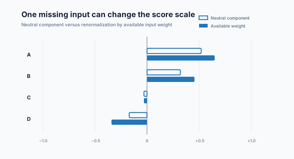
Three-input composite with incomplete coverage
| Security | Input 1 | Input 2 | Input 3 | Neutral-component score | Available-weight score |
|---|---|---|---|---|---|
| A | +0.8 | +0.4 | missing | +0.520 | +0.650 |
| B | +0.4 | missing | +0.6 | +0.320 | +0.457 |
| C | −0.1 | +0.2 | −0.2 | −0.030 | −0.030 |
| D | missing | −0.5 | −0.1 | −0.170 | −0.340 |
For A, neutral component treatment gives
\[s_A^{\mathrm{neutral}} =0.50(0.8)+0.30(0.4)+0.20(0)=0.520.\]
The available inputs account for absolute weight \(0.50+0.30=0.80\), so
\[s_A^{\mathrm{available}} =\frac{0.520}{0.80}=0.650.\]
D illustrates the risk of renormalization. Its two observed components supply only half of the intended model weight, and dividing by \(0.50\) doubles the magnitude from \(-0.170\) to \(-0.340\). A minimum-coverage rule could instead make D ineligible.
Python calculation
import pandas as pd

inputs = pd.DataFrame(
    {
        "input_1": [0.8, 0.4, -0.1, None],
        "input_2": [0.4, None, 0.2, -0.5],
        "input_3": [None, 0.6, -0.2, -0.1],
    },
    index=["A", "B", "C", "D"],
)
weights = pd.Series({"input_1": 0.50, "input_2": 0.30, "input_3": 0.20})

available = inputs.notna()
input_coverage = available.mean()                        # 0.75 on every input
complete_case_coverage = available.all(axis=1).mean()    # 0.25

neutral_score = inputs.fillna(0).mul(weights).sum(axis=1)
available_weight = available.mul(weights.abs()).sum(axis=1)
renormalized_score = neutral_score / available_weight

result = pd.DataFrame(
    {
        "neutral_score": neutral_score,
        "available_weight": available_weight,
        "renormalized_score": renormalized_score,
    }
)
Positive, zero, and missing are separate states
A positive factor component supports the recorded direction, and a negative component opposes it. Zero ordinarily represents the cross-sectional centre or a measured neutral value. Missing means the system lacks a valid observation under the timing and quality rules.
If neutral treatment maps missing to zero for calculation, the availability indicator still needs to be retained. Otherwise portfolio review cannot tell a balanced signal from an incomplete one.
Where this goes wrong
Filling on the wrong scale
For a valuation ratio, count, price, or return, a raw zero usually carries a specific economic meaning, so neutrality belongs on the normalized scale rather than in the raw field. Available-weight renormalization has the mirror failure: applied without limits it can reduce a multi-input factor to a single input for poorly covered securities, which is what required inputs, a minimum component count, and a minimum represented weight exist to prevent.
Imputing with information you did not have
Group membership and peer values must both be as they stood at the observation time. Current sector classifications and restated fundamentals introduce look-ahead bias into every historical date they touch. An operational failure belongs on a different path altogether: a feed that times out should raise freshness and quality controls, because routing it into the imputation rule turns an infrastructure problem into live position changes without anyone being told.
Informative missingness
Absence is informative when it correlates with the securities themselves rather than arriving at random. Young companies, distressed issuers, and thinly traded assets tend to be missing systematically, so an imputed factor can inherit a size, sector, or liquidity bias even when the filled values look neutral. The measurement consequence follows from the same fact: an improving IC may only mean the factor became available for the easier names. Store coverage, coverage by group, and the evaluation universe beside every result.
Signal and portfolio consequences
Each policy changes ranks, information coefficient, turnover, and exposure. Complete-case evaluation measures performance among covered securities. Neutral treatment preserves broader coverage while shrinking scores for names with missing components. Available-weight treatment preserves magnitude but changes the effective input mix.
Portfolio construction can include a coverage penalty, cap positions with imputed inputs, or require a minimum confidence score. Comparing performance on the intersection of valid observations helps determine whether an apparent improvement comes from the model or from the sample.
Frequently asked questions
Is median imputation always neutral?
It is central within the chosen peer group on that date. After later transforms or global ranking it may not equal zero, and securities that are absent systematically can still create exposure.
Do sophisticated imputation methods beat simple ones?
Not reliably. Chen and McCoy (2024) characterize the missing values across 159 cross-sectional predictors and find that imputing with the cross-sectional mean performs about as well as expectation-maximization for machine-learning portfolios, because absence arrives in large blocks organized by time and by data source, so the observed data says little about what is missing. Freyberger and co-authors (2025) obtain improved out-of-sample predictability by handling conditional mean imputation inside the estimator instead of as a pre-processing step. Both results point the effort at the timing and eligibility rules ahead of the interpolation method.
Should missing values receive the worst rank?
Only when absence itself has a stated adverse interpretation supported by the research design. Otherwise the rule invents a negative signal.
Can absence itself be a signal?
Yes. If it carries repeatable information, test the availability indicator as its own feature, point in time. That keeps the observed characteristic and the hypothesis about absence separately identifiable.
What should be stored with each score?
At minimum: source timestamps, available-input mask, imputation flags, input ages, represented weight, universe eligibility, and the factor version.
Next reading
- What Is Cross-Sectional Ranking?
- Should Alpha Factors Be Z-Scored or Ranked?
- How to compose registered signals into a factor
Sources
- Joachim Freyberger, Björn Höppner, Andreas Neuhierl, and Michael Weber, “Missing Data in Asset Pricing Panels”, The Review of Financial Studies 38(3), 2025, 760–802.
- Andrew Y. Chen and Jack McCoy, “Missing values handling for machine learning portfolios”, Journal of Financial Economics 155, 2024, article 103815.
- Roderick J. A. Little and Donald B. Rubin, Statistical Analysis with Missing Data, Wiley, 3rd edition, 2019 (ISBN 978-0-470-52679-8) — the foundational treatment of the MCAR, MAR, and MNAR distinction used above.
- pandas missing-data documentation
This walkthrough is for research and educational purposes. It illustrates how strategynet.ai organizes signal evidence into factors and scenarios. It provides no recommendation, investment advice, or instruction to trade any security.
Back to Insights