What Is a Trading Signal in Quantitative Finance?

A trading signal is a dated, reproducible rule that converts information available at a decision time into a forecast or an action-relevant score. In cross-sectional research, it usually assigns one value to every eligible security. The value may forecast relative return, risk, volatility, liquidity, or the probability of an event over a stated horizon.

The signal is one stage in a longer process. Market data supplies observations; transformations create comparable features; the signal gives those features a forecast direction; a factor definition produces the signal repeatedly across securities and dates; and portfolio construction determines holdings. Keeping these records separate makes it possible to learn whether an idea failed in its data, its forecast, or its implementation.

Mathematical definition

Let \(\mathcal{I}_t\) contain the information that was available by observation time \(t\), and let \(U_t\) be the eligible universe at that time. A cross-sectional signal is a function

\[s_{i,t} = g(i,\mathcal{I}_t;\theta_v), \qquad i\in U_t,\]

where \(g\) is the recorded calculation, \(\theta_v\) contains the parameters for version \(v\), and \(s_{i,t}\) is the output for security \(i\). The definition also needs a forecast target, such as the subsequent return

\[R_{i,t+1:t+h} = \frac{P_{i,t+h}}{P_{i,t}}-1,\]

where \(h\) is the horizon and the first executable return begins after the signal cutoff. For an intraday signal, the price and execution conventions would be more specific than the closing-price notation above.

The complete signal record therefore includes the source fields, availability lags, eligible universe, transformations, parameters, orientation, cutoff, refresh schedule, missing-value rule, and forecast horizon. A formula without those conventions cannot be reproduced point in time.

Observation, feature, signal, factor, and trade

These terms describe different objects:

Industry usage is not perfectly uniform; researchers often use signal and factor for the same score column. The distinctions above are operational. They identify which object was observed, which rule generated it, and whether portfolio weights have actually been calculated.

Crowding worked example

Consider the hypothesis that short-position pressure and weak recent price action identify securities with elevated squeeze potential. A factor cannot consume that sentence. It needs measured inputs.

For security \(i\), calculate

\[DTC_i=\frac{\text{short interest}_i}{\text{20-day average volume}_i}, \qquad SVR_i=\frac{\text{reported short-sale volume}_i} {\text{corresponding reported volume}_i},\]

and the recent five-day return \(r_i^{(5)}\). Convert each field to a centred cross-sectional rank \(q(\cdot)\) between \(-1\) and \(+1\), then define

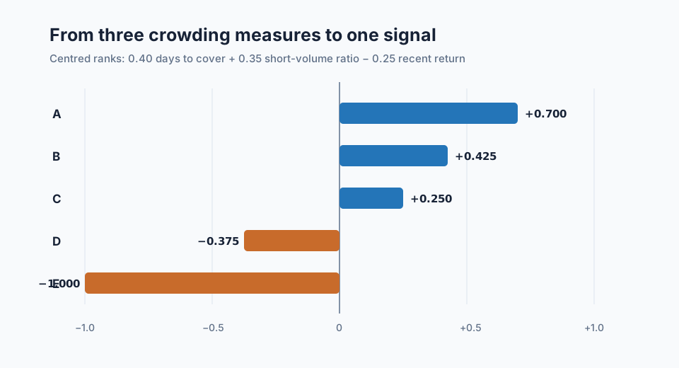
\[s_i = 0.40q(DTC_i)+0.35q(SVR_i)-0.25q(r_i^{(5)}).\]

In the five-security example developed in What Is Factor Crowding?, security A has 10 days to cover, a 45% short-volume ratio, and a five-day return of \(-2\%\). Its centred ranks are \(+1.00\), \(+0.50\), and \(-0.50\), so

\[s_A =0.40(1.00)+0.35(0.50)-0.25(-0.50) =0.700.\]

The sentence about squeeze pressure has now become one dated number. Repeating the same calculation for A through E produces scores of \(0.700\), \(0.425\), \(0.250\), \(-0.375\), and \(-1.000\). That vector is the signal cross-section at the observation time.

Python example

import pandas as pd

features = pd.DataFrame(
    {
        "days_to_cover": [10.0, 6.0, 3.0, 2.0, 1.0],
        "short_volume_ratio": [0.45, 0.60, 0.30, 0.20, 0.10],
        "return_5d": [-0.02, 0.04, -0.08, 0.01, 0.08],
    },
    index=["A", "B", "C", "D", "E"],
)

def centred_rank(series):
    rank = series.rank(method="average")
    return 2 * (rank - 1) / (series.count() - 1) - 1

normalized = features.apply(centred_rank)
signal = (
    0.40 * normalized["days_to_cover"]
    + 0.35 * normalized["short_volume_ratio"]
    - 0.25 * normalized["return_5d"]
)

print(signal.round(3))

This example uses average ranks, requires all three inputs, and calculates the cross-section at one time. A deployed version would also check source timestamps and minimum coverage before emitting a value.

Positive, zero, and negative values

The meaning of the sign comes from the declared orientation. Under this crowding definition, a positive score means the measured evidence lies above the cross-sectional centre for squeeze pressure. A negative score means it lies below the centre. A score near zero can mean that every component is ordinary, or that unusually high and low components offset one another.

A positive score is not automatically a buy order. It becomes actionable only after the forecast direction is supported, the expected benefit is compared with risk and cost, and the portfolio rule decides a weight. A risk system could also use the same positive score to reduce an existing short rather than open a long position.

How a signal becomes a factor

One score vector is a set of signal observations. The factor is the stable rule that generates those observations on a schedule:

\[\mathbf{s}_t = \left(s_{1,t},s_{2,t},\ldots,s_{N_t,t}\right)^\top.\]

The version changes if the input set, lag, universe, normalization, weights, orientation, or horizon changes. This prevents results obtained from one rule from being attributed to a later rule with the same display name.

Predictive evaluation compares the dated cross-section with outcomes observed afterward. Rank information coefficient is one such test:

\[IC_t = \operatorname{corr}_{i\in U_t} \left( \operatorname{rank}(s_{i,t}), \operatorname{rank}(R_{i,t+1:t+h}) \right).\]

Repeated through time, the calculation shows whether the ordering persists, changes across regimes, or depends on a small part of the universe. Quantile spreads, turnover, coverage, tail outcomes, and marginal information beyond existing factors answer other parts of the evaluation.

How the factor becomes a portfolio

A factor-mimicking portfolio chooses holdings with exposure to the signal while controlling unwanted risks. In compact form,

\[\begin{aligned} \min_{\mathbf{w}_t}\quad & \frac{1}{2}\mathbf{w}_t^\top\Sigma_t\mathbf{w}_t \\ \text{subject to}\quad & \mathbf{w}_t^\top\mathbf{s}_t=1, \\ & \mathbf{w}_t^\top\mathbf{1}=0, \\ & \mathbf{w}_t^\top B_t=\mathbf{0}. \end{aligned}\]

Here \(\Sigma_t\) is the covariance estimate and \(B_t\) contains exposures such as sectors, market beta, and size that the construction intends to neutralize. Position, liquidity, turnover, and borrowing constraints can be added. The result is a return history for a defined factor portfolio, which can be tested walk forward and compared with other candidates.

A client portfolio requires another decision. It may combine several validated factor portfolios, current forecasts, covariance, costs, and mandate-specific limits. A successful signal supplies evidence to that process; it does not determine the final holdings by itself.

Common signal mistakes

Using information before it was available

Fundamental releases, position reports, and revised macroeconomic series have effective dates and availability dates. The signal may use only the version known at its cutoff.

Omitting the horizon

A predictor can have positive association with next-day returns and negative association with next-month returns. A signal described without its target horizon leaves its central claim undefined.

Combining incompatible scales

Adding a dollar value, a percentage, and a count gives the largest numerical unit control of the result. Orientation and normalization precede composition.

Filling missing values without economic justification

Zero can represent a real neutral observation, while a missing value means the observation was unavailable or invalid. Conflating them changes both coverage and rank.

Estimating parameters on the full history

Weights, thresholds, and transformations selected using future outcomes leak test information into past signals. Adaptive parameters need a training window ending before each observation.

Equating a score with an order

Forecast strength, covariance, liquidity, current holdings, transaction costs, and constraints determine whether a score leads to a trade. The signal record should remain valid even when the portfolio correctly chooses no transaction.

Relationship to adjacent terms

An alpha factorAlpha factorA measurable security characteristic or signal used to forecast relative future returns.Open glossary entry → is a signal whose stated purpose is to rank expected relative returns. Some signals instead forecast volatility, liquidity, drawdown, or event probability. Factor exposureFactor exposureThe sensitivity of a security or portfolio to a specified factor, estimated from holdings, characteristics, or a return model.Open glossary entry → measures how strongly a security or portfolio represents a factor, while information coefficientInformation coefficient (IC)The cross-sectional correlation between a signal score and a subsequent return. Rank IC uses ranked values and measures whether the signal orders securities correctly.Open glossary entry → measures the association between a signal cross-section and later returns.

Cross-sectional ranking, winsorization, z-scoring, neutralization, and missing data rules are transformations or controls used within the pipeline. They do not supply the economic hypothesis on their own.

Frequently asked questions

Is a technical indicator a trading signal?

It becomes one when its inputs, calculation, timing, orientation, and forecast horizon are specified. A chart label such as “momentum” is too broad to reproduce.

Can a signal contain several factors?

A composite signal can combine several primitive signals. If the result has a stable definition and produces one score per security and date, it can be registered and evaluated as a factor in its own right.

Does every signal have to be cross-sectional?

No. A time-series signal may forecast one instrument through time, and an event signal may forecast an outcome probability. Cross-sectional signals are particularly useful when the decision is how to allocate among many securities at the same time.

When is the factor ready for portfolio use?

After point-in-time materialization and walk-forward evaluation show that its behaviour is sufficiently stable for the intended use, including costs, turnover, coverage, concentration, and tail risk. The acceptance criteria should be chosen before the holdout result is known.

Next reading

• What Is Factor Crowding?
• Alpha factor: a cross-sectional signal that ranks expected returns
• How to compose registered signals into a factor

Sources

• Richard C. Grinold and Ronald N. Kahn, Active Portfolio Management: A Quantitative Approach for Producing Superior Returns and Controlling Risk, McGraw-Hill, 2nd edition, 2000 (ISBN 978-0-07-024882-3).
• FINRA, “Short Interest – What It Is, What It Is Not”.
• FINRA, “Understanding Short Sale Volume Data on FINRA's Website”.
• Dong Lou and Christopher Polk, “Comomentum: Inferring Arbitrage Activity from Return Correlations”, The Review of Financial Studies, 2022.