
What Is Alpha Uncertainty?
Alpha uncertainty describes the imprecision of an expected-return forecast. It depends on the data, estimation method, sample size, market conditions, and forecast horizon. Incorporating that uncertainty into portfolio construction allows position sizes to reflect the strength of the evidence behind a forecast.
This article explains uncertainty for security and factor-portfolio forecasts, works through an allocation example, and shows how uncertainty enters a robust optimization objective.
Forecast and error
Let \(\widehat{\boldsymbol\alpha}_t\) be the vector of expected returns supplied to the portfolio calculation at time \(t\). Write
\[\widehat{\boldsymbol\alpha}_t = \boldsymbol\alpha_t+\boldsymbol\varepsilon_t,\]
where \(\boldsymbol\alpha_t\) is the unknown conditional expected return and \(\boldsymbol\varepsilon_t\) is estimation error. The error can have a nonzero mean \(\mathbf m_{\varepsilon,t}\) and covariance \(\Omega_{\varepsilon,t}\). The diagonal elements of \(\Omega_{\varepsilon,t}\) measure uncertainty in each forecast; its off-diagonal elements record errors that tend to occur together.
Historical forecast error becomes observable after the evaluation horizon:
\[\mathbf e_{t+h} = \widehat{\boldsymbol\alpha}_t-\mathbf r_{t\rightarrow t+h}.\]
Those completed errors can estimate bias and covariance, provided each observation uses the forecast actually available at \(t\), the matching realized return, and the same horizon and units. Overlapping horizons require a dependence-aware estimate rather than being treated as independent records.
An ellipsoidal uncertainty set
A common robust formulation places the unknown expected-return vector in an ellipsoid around the estimate:
\[\mathcal U_t(k) = \left\{ \mathbf a: (\mathbf a-\widehat{\boldsymbol\alpha}_t)^{\mathsf T} \Omega_{\varepsilon,t}^{-1} (\mathbf a-\widehat{\boldsymbol\alpha}_t) \le k^2 \right\}.\]
\(k\) controls the radius. A larger value asks the portfolio to withstand a wider set of forecast errors. When the uncertainty covariance is positive definite, the lowest expected portfolio return inside the ellipsoid has a closed form:
\[\min_{\mathbf a\in\mathcal U_t(k)} \mathbf w^{\mathsf T}\mathbf a = \mathbf w^{\mathsf T}\widehat{\boldsymbol\alpha}_t -k\sqrt{ \mathbf w^{\mathsf T} \Omega_{\varepsilon,t} \mathbf w }.\]
The square-root term is the standard deviation of portfolio forecast error. It depends on the positions and on the correlation between their errors. A robust mean-variance problem can therefore be written
\[\max_{\mathbf w\in\mathcal W_t} \left\{ \mathbf w^{\mathsf T}\widehat{\boldsymbol\alpha}_t -k\sqrt{\mathbf w^{\mathsf T}\Omega_{\varepsilon,t}\mathbf w} -\frac{\lambda}{2} \mathbf w^{\mathsf T}\Sigma_t\mathbf w \right\},\]
where \(\Sigma_t\) is the covariance of investment returns, \(\lambda\) is risk aversion, and \(\mathcal W_t\) contains the budget, exposure, liquidity, and position constraints. The two covariance matrices answer different questions: \(\Sigma_t\) estimates variability in portfolio returns, while \(\Omega_{\varepsilon,t}\) estimates uncertainty in the expected-return input.
A two-factor example
Suppose an allocation is being made between two factor portfolios. Their annual expected returns are 8% and 5%. Forecast-error standard deviations are 4% and 2%, and their error correlation is 0.25, giving
\[\widehat{\boldsymbol\alpha} = \begin{bmatrix}0.08\\0.05\end{bmatrix}, \qquad \Omega_\varepsilon = \begin{bmatrix} 0.0016 & 0.0002\\ 0.0002 & 0.0004 \end{bmatrix}.\]
Set \(k=1.645\) for this illustration. This number resembles a one-sided 95% normal quantile, although an empirical application should calibrate the radius from its own completed forecast errors rather than attach a probability to the ellipsoid automatically.
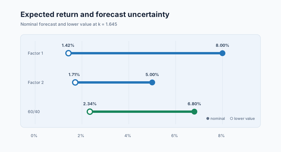
Expected return and uncertainty for three candidate allocations
| Weights in factors 1 and 2 | Expected return | Error standard deviation | Robust lower value |
|---|---|---|---|
| (1.0, 0.0) | 8.00% | 4.00% | 1.42% |
| (0.0, 1.0) | 5.00% | 2.00% | 1.71% |
| (0.6, 0.4) | 6.80% | 2.71% | 2.34% |
The first factor has the largest nominal forecast and the lowest robust value because its forecast is less precise. The 60/40 allocation has forecast-error variance
\[0.6^2(0.0016) +2(0.6)(0.4)(0.0002) +0.4^2(0.0004) =0.000736,\]
so its error standard deviation is 2.71%. Its robust value is \(6.80\%-1.645(2.71\%)=2.34\%\), the largest of the three candidates. This calculation only compares forecast uncertainty; an allocation decision would also include return covariance and the other portfolio constraints.
import numpy as np

alpha = np.array([0.08, 0.05])
omega_error = np.array(
    [
        [0.0016, 0.0002],
        [0.0002, 0.0004],
    ]
)
k = 1.645

candidates = {
    "factor 1": np.array([1.0, 0.0]),
    "factor 2": np.array([0.0, 1.0]),
    "60/40": np.array([0.6, 0.4]),
}

for name, weight in candidates.items():
    expected = weight @ alpha
    error_sd = np.sqrt(weight @ omega_error @ weight)
    robust_value = expected - k * error_sd
    print(name, expected, error_sd, robust_value)
Interpreting the lower value
A positive robust value means the expected portfolio return remains positive at the adverse boundary of the stated uncertainty set. A zero value places that boundary at zero expected return. A negative value means the uncertainty set contains expected-return vectors under which the portfolio's expected return is negative.
These signs describe the model and radius used in the calculation. They do not give the probability of a positive realized return unless the uncertainty set, error distribution, and calibration procedure support that interpretation. A portfolio can have a positive robust expected value and subsequently lose money; realized returns contain both forecast error and investment risk.
Estimating forecast uncertainty
For a repeated factor forecast, one practical route is to retain every dated forecast and its later realized return, then estimate the error mean and covariance over a trailing or expanding window. The estimate can be diagonal when the history is short, shrunk toward a structured target when the full matrix is noisy, or modeled from a smaller set of error factors.
The observation unit must match the decision. A security-level model needs errors across securities and time. An allocator combining factor-mimicking portfolios needs the errors of those factor-return forecasts. A cross-sectional rank score has no expected-return unit until it has been calibrated; applying a percentage-return uncertainty matrix directly to raw ranks mixes scales.
The radius \(k\) should be chosen before the reporting interval. Useful checks include the historical coverage of the uncertainty set, results across several predeclared radii, weight stability, forecast concentration, and performance in market states that were scarce in the estimation sample.
Common implementation mistakes
Reusing return covariance as forecast-error covariance
Volatile investments can have precise forecasts, and quiet investments can have unreliable forecasts. Estimate \(\Sigma_t\) and \(\Omega_{\varepsilon,t}\) from the quantities each matrix is meant to describe.
Measuring error with revised or mismatched forecasts
The archived forecast must be the value known at the portfolio date. Its target return must use the same horizon, currency, corporate-action treatment, and universe convention.
Ignoring correlated mistakes
Two forecasts derived from similar data or economic relationships can fail together. A diagonal error matrix overstates the diversification obtained by combining them when their errors are positively correlated.
Selecting the radius from the final results
Choosing \(k\) because it gives the best completed backtest turns the uncertainty setting into another fitted parameter. Calibrate it in a training interval and carry it unchanged into the next evaluation interval.
Penalizing uncertainty after weights are chosen
An after-the-fact haircut measures a completed portfolio but cannot change its concentration. The robust term belongs inside the optimization when the purpose is to influence holdings.
Treating uncertainty control as a substitute for research quality
Robust construction cannot repair look-ahead bias, missing point-in-time data, unstable universes, or a forecast with no repeatable evidence. It begins after the forecast record has been made reproducible.
How it enters signal and portfolio evaluation
StrategyNet users can start with registered factors, add their own signals, and combine them into new factors. Each resulting forecast can be evaluated over time and converted into one or more factor-mimicking portfolios. The software can then compare a nominal allocation with constructions that use estimated forecast-error bias, covariance, or scenario losses.
The useful comparison keeps the universe, forecast version, rebalance dates, return covariance, and portfolio constraints fixed. Report expected return, realized risk, drawdown, turnover, concentration, and the fraction of subsequent errors contained by the selected uncertainty rule. This reveals whether the uncertainty control improved stability and where it gave up forecast exposure.
Frequently asked questions
Is alpha uncertainty the same as alpha volatility?
Alpha uncertainty concerns error in the expected-return estimate. Alpha volatility is sometimes used for variability in realized active returns or in a time series of forecasts. The underlying quantity should be stated whenever the phrase is used.
Does more historical data always reduce uncertainty?
More relevant observations can improve precision, but old observations may describe a different regime or process. Sample length, structural change, and the effective number of independent observations all matter.
Can uncertainty be estimated for a newly created factor?
Only to the extent that its historical definition can be reconstructed point in time. A genuinely new signal may need a conservative prior, related-factor evidence, or tighter allocation bounds until enough completed forecasts exist.
Why use an ellipsoid?
It represents correlated forecast errors compactly and produces a tractable second-order cone problem. Box sets, scenario sets, distributionally robust methods, and direct forecast-error constraints are alternatives with different assumptions.
Next reading
- Does Forecast-Error Control Stabilize Portfolios?
- How Do Multiple Risk Models Enter Portfolio Construction?
- Robust Portfolio Optimization
Sources
- Stefano Benati and Eduardo Conde, “A Relative Robust Approach on Expected Returns with Bounded CVaR for Portfolio Selection”, European Journal of Operational Research, 2022. Studies portfolio choice under uncertain expected returns and economic scenarios.
- Man Yiu Tsang, Tony Sit, and Hoi Ying Wong, “Robust Portfolio Optimization with Respect to Spectral Risk Measures Under Correlation Uncertainty”, Applied Mathematics & Optimization, 2022. Extends portfolio ambiguity to uncertain correlations and multistage decisions.
- Fiona Kolbert and Laurence Wormald, “Robust Portfolio Optimization Using Second-Order Cone Programming”, in Optimizing Optimization, 2010.
- Donald Goldfarb and Garud Iyengar, “Robust Portfolio Selection Problems”, Mathematics of Operations Research, 2003. Included as a foundational treatment of ellipsoidal parameter uncertainty in portfolio selection.
This walkthrough is for research and educational purposes. It illustrates how strategynet.ai organizes signal evidence into factors and scenarios. It provides no recommendation, investment advice, or instruction to trade any security.
Back to Insights