
What Is the Fundamental Law of Active Management?
The Fundamental Law of Active Management relates forecasting skill, the number of independent investment decisions, and expected risk-adjusted performance. Its generalized form also accounts for how closely portfolio positions reflect the forecasts. The relationship helps investment teams assess where better research, broader opportunities, or changes to constraints could improve a strategy.
This article develops the approximation, works through numerical examples, and explains the assumptions that govern its use in portfolio design.
Original and generalized forms
The original expression is
\[IR\approx IC\sqrt{BR},\]
where:
- \(IR\) is the expected Information Ratio of active return to active risk;
- \(IC\) is the expected correlation between forecasts and subsequent returns;
- \(BR\) is the number of independent decisions over the same measurement period.
Portfolio constraints can prevent holdings from aligning fully with forecasts. A generalized form introduces the transfer coefficient:
\[IR\approx IC\times TC\times\sqrt{BR}.\]
\(TC\) is the correlation between risk-adjusted forecasts and risk-adjusted active positions. Under an ideal unconstrained implementation, \(TC\) approaches one.
Worked example
Suppose a process has:
\[IC=0.06, \qquad BR=100\text{ independent decisions per year}, \qquad TC=0.50.\]
Its potential annual Information Ratio under the generalized law is
\[IR \approx 0.06\times0.50\times\sqrt{100} =0.30.\]
If the portfolio targets annual active risk of \(4\%\), the corresponding expected active return is
\[\mathbb{E}[R_A] \approx IR\times\sigma_A =0.30\times4\% =1.20\%.\]
This last multiplication changes aggressiveness, not information quality. A higher active-risk target scales both expected active return and risk under the linear approximation.
How each component changes potential Information Ratio
| IC | Effective breadth | Transfer coefficient | Potential IR |
|---|---|---|---|
| 0.03 | 100 | 0.50 | 0.15 |
| 0.06 | 100 | 0.50 | 0.30 |
| 0.06 | 25 | 0.50 | 0.15 |
| 0.06 | 100 | 0.80 | 0.48 |
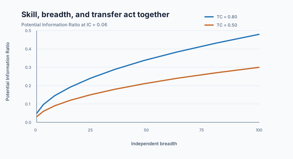
Doubling IC doubles the approximation. Reducing breadth from 100 to 25 halves it because breadth enters through its square root. Increasing transfer from \(0.50\) to \(0.80\) raises the fraction of forecast information reflected in the positions.
Python calculation
import numpy as np

information_coefficient = 0.06
breadth = np.array([1, 4, 9, 16, 25, 36, 49, 64, 81, 100])

ir_at_tc_50 = information_coefficient * 0.50 * np.sqrt(breadth)
ir_at_tc_80 = information_coefficient * 0.80 * np.sqrt(breadth)

print(np.round(ir_at_tc_50, 3))
# [0.03 0.06 0.09 0.12 0.15 0.18 0.21 0.24 0.27 0.30]
The role of information coefficient
IC measures forecast skill. In cross-sectional factor research, it is commonly the date-level correlation between security scores and later returns, averaged over a history. The IC convention, horizon, universe, timing, and dependence adjustment must match the decision process represented by breadth.
An IC estimate selected from many tested signals is optimistic unless multiple testing and holdout design are addressed. The law treats skill as known and repeatable; empirical research must estimate its uncertainty.
The role of breadth
Breadth counts independent decisions during the measurement period. It is not the number of securities, rows, or rebalances. Common factor exposures, correlated signals, overlapping returns, and persistent holdings reduce effective breadth.
If ten equally important decisions have pairwise correlation \(0.20\), their variance-equivalent breadth is only
\[\frac{10}{1+9(0.20)}=3.57.\]
Using the raw count in the law would overstate the opportunity set.
The role of transfer coefficient
The transfer coefficient measures alignment between risk-adjusted forecasts and active positions. Long-only rules, sector neutrality, factor limits, turnover controls, position caps, and liquidity constraints can reduce it.
A lower transfer coefficient can be a rational cost of controlling an unacceptable risk. The useful question is whether each constraint removes more forecast alignment than its risk or implementation benefit justifies.
Positive, zero, and negative values
With positive breadth, the sign of potential IR follows the product \(IC\times TC\). Positive IC and positive transfer imply positive expected active performance under the selected direction. IC near zero implies little potential IR regardless of breadth. A negative IC indicates that forecasts tend to order returns in the opposite direction.
Transfer is usually intended to be positive. A negative value indicates that positions tend to oppose forecasts. Breadth is non-negative and enters through its square root.
Assumptions behind the approximation
The simple form relies on assumptions that include:
- forecast correlations are stable and measured on the correct horizon;
- breadth represents independent or properly adjusted decisions;
- forecast skill is sufficiently similar across the decisions being aggregated;
- positions are sized in a manner consistent with forecasts and risk;
- covariance and transfer are measured without material error;
- costs, nonlinear payoffs, tail dependence, and regime changes do not dominate.
Violations do not make the framework useless. They identify which additional measurements the actual research process must supply.
Common implementation mistakes
Treating the formula as a performance forecast
The output is a structural approximation. A walk-forward portfolio test is needed to estimate realized return, risk, drawdown, and cost.
Counting correlated holdings as independent breadth
Many securities can express one sector, duration, volatility, or liquidity view. Dependence belongs in the breadth estimate.
Combining IC and breadth from different horizons
A one-day IC cannot be paired casually with annual decision counts based on overlapping monthly positions. Timing conventions must describe one process.
Omitting transfer while imposing strong constraints
The original law can overstate attainable performance when holdings depart materially from forecasts.
Applying a selected in-sample IC without shrinkage
Search and estimation error make the observed IC an uncertain estimate. Point-in-time shrinkage and clean holdouts are required before allocation.
Ignoring transaction costs
High nominal breadth often requires frequent or diffuse trading. Gross information does not ensure positive net active return.
Use in signal and portfolio evaluation
The framework helps locate a weak link. Low IC directs attention to the signal and labels. Low effective breadth suggests duplicated opportunities or overlapping timing. Low transfer points to constraints and instrument choice. A respectable product of all three can still be consumed by costs or tail risk, which remain separate tests.
For a StrategyNet factor portfolio, the components can be estimated from the stored signal history, completed forward returns, factor-portfolio correlations, and constrained holdings. The final evaluation retains the empirical return history beside the law's diagnostic decomposition.
Frequently asked questions
Does doubling the number of securities double Information Ratio?
No. Even independent breadth enters through a square root, and securities are rarely independent decisions.
Is a low IC useless?
Not necessarily. A small persistent IC applied across substantial independent breadth can support useful risk-adjusted performance. Costs and implementation still determine economic value.
Can transfer coefficient exceed one?
As a correlation under the standard definition, it lies between \(-1\) and \(+1\). Apparent values outside that range indicate a different measure or a calculation error.
Where does active risk appear?
Information Ratio is expected active return divided by active risk. Choosing an active-risk target scales the expected active return after the law estimates the risk-adjusted opportunity.
Next reading
- What Is Factor Breadth?
- What Is the Transfer Coefficient?
- Information Coefficient vs Information Ratio
Sources
- Richard C. Grinold, “The Fundamental Law of Active Management”, The Journal of Portfolio Management, 1989.
- Roger G. Clarke, Harindra de Silva, and Steven Thorley, “Portfolio Constraints and the Fundamental Law of Active Management”, Financial Analysts Journal, 2002.
This walkthrough is for research and educational purposes. It illustrates how strategynet.ai organizes signal evidence into factors and scenarios. It provides no recommendation, investment advice, or instruction to trade any security.
Back to Insights