
What Is an Eigenportfolio?
An eigenportfolio takes its weights from an eigenvector of a return covariance or correlation matrix. It represents a pattern of shared movement among assets; the associated eigenvalue measures the variance captured by that pattern. Portfolio researchers use these patterns to examine concentration and identify the main sources of variation in a return history.
This article works through a two-asset example, explains the common and spread portfolios it produces, and discusses how to interpret and use the resulting weights. Economic interpretations depend on the sample and can change through time.
Mathematical definition
For an \(N\times N\) covariance matrix \(\Sigma\), eigenvalue \(\lambda_k\) and unit-length eigenvector \(\mathbf{v}_k\) satisfy
\[\Sigma\mathbf{v}_k = \lambda_k\mathbf{v}_k, \qquad \mathbf{v}_k^\top\mathbf{v}_k=1.\]
For a symmetric covariance matrix, the eigenvectors can be chosen orthonormal:
\[\mathbf{v}_j^\top\mathbf{v}_k=0 \quad\text{for }j\ne k.\]
If returns are centred and the eigenvector is used directly as a weight vector, the unit-norm eigenportfolio return is
\[f_{k,t}=\mathbf{v}_k^\top\mathbf{r}_t\]
with variance
\[\operatorname{Var}(f_k) = \mathbf{v}_k^\top\Sigma\mathbf{v}_k =\lambda_k.\]
An investable portfolio normally needs another normalization for gross, net, volatility, or capital exposure.
Two-asset worked example
Suppose two assets each have variance \(0.04\) and covariance \(0.03\):
\[\Sigma = \begin{bmatrix} 0.04 & 0.03\\ 0.03 & 0.04 \end{bmatrix}.\]
The eigenpairs are
\[\lambda_1=0.07, \qquad \mathbf{v}_1=\frac{1}{\sqrt{2}} \begin{bmatrix}1\\1\end{bmatrix},\]
and
\[\lambda_2=0.01, \qquad \mathbf{v}_2=\frac{1}{\sqrt{2}} \begin{bmatrix}1\\-1\end{bmatrix}.\]
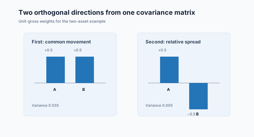
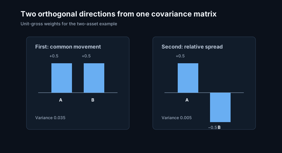
The first direction moves both assets together and captures seven times the variance of the second. The second is a spread between them.
For a unit-gross presentation, divide each vector by the sum of its absolute weights. The portfolios become \((0.5,0.5)\) and \((0.5,-0.5)\). Their variances are \(0.035\) and \(0.005\), respectively; the rescaling halves each unit-norm variance because the weight vector is divided by \(\sqrt{2}\).
If the next returns are \(+4\%\) and \(+2\%\), the unit-gross common portfolio earns
\[0.5(4\%)+0.5(2\%)=3\%,\]
and the unit-gross spread earns
\[0.5(4\%)-0.5(2\%)=1\%.\]
Two covariance eigenportfolios
| Portfolio | Unit-gross weights | Variance | Interpretation in this sample |
|---|---|---|---|
| First | (+0.5, +0.5) | 0.035 | Common movement |
| Second | (+0.5, −0.5) | 0.005 | Relative spread |
Python calculation
import numpy as np

covariance = np.array(
    [
        [0.04, 0.03],
        [0.03, 0.04],
    ]
)

eigenvalue, eigenvector = np.linalg.eigh(covariance)
order = np.argsort(eigenvalue)[::-1]
eigenvalue = eigenvalue[order]
eigenvector = eigenvector[:, order]

# Eigenvector signs are arbitrary; orient the first asset positively for display.
eigenvector *= np.sign(eigenvector[0])
unit_gross_weight = eigenvector / np.abs(eigenvector).sum(axis=0)

print(np.round(eigenvalue, 2))
print(np.round(unit_gross_weight, 2))
Covariance PCA and correlation PCA
Covariance PCA gives more influence to assets with larger return variance. Correlation PCA first standardizes each return by its volatility and studies the dependence structure on a common scale. The two methods produce different eigenvectors.
When an eigenvector \(\mathbf{v}_k\) is estimated from a correlation matrix of standardized returns, a return portfolio in original asset units may use volatility-adjusted weights proportional to
\[w_{i,k}\propto\frac{v_{i,k}}{\sigma_i}.\]
The final normalization must then state gross, net, and volatility conventions. Calling both the correlation eigenvector and its volatility-adjusted asset weights “the eigenportfolio” without explanation creates avoidable ambiguity.
Positive and negative weights
Positive and negative eigenvector elements show which assets move on opposite sides of that statistical direction. The entire vector can be multiplied by \(-1\) without changing the eigenvalue or the represented subspace. Its sign is therefore arbitrary until an orientation convention is imposed.
Eigenvalues of a valid covariance matrix are non-negative. A materially negative estimated eigenvalue indicates that the matrix is not positive semidefinite, often because of inconsistent data, pairwise estimation, or numerical error.
Eigenportfolios as statistical factors
The leading eigenportfolios provide a compact statistical factor model. If \(K<N\) leading directions are retained, returns can be approximated by
\[\mathbf{r}_t \approx V_K\mathbf{f}_t+\boldsymbol{\varepsilon}_t,\]
where \(V_K\) contains the retained eigenvectors and \(\boldsymbol{\varepsilon}_t\) is residual return. The model separates common variation from asset-specific or lower-variance directions under the estimated sample covariance.
Residuals can be studied for relative-value or mean-reversion hypotheses, but PCA alone supplies no forecast. Any trading signal built from a residual needs its own timing, economic rationale, parameter estimation, and walk-forward evaluation.
Common implementation mistakes
Using future returns in the covariance window
Historical eigenportfolios must be estimated using returns available before the rebalance and then held fixed over the evaluation period.
Ignoring eigenvector sign and ordering instability
Signs can flip between runs, and nearby eigenvalues allow eigenvectors to rotate substantially. Align directions by subspace or a recorded orientation before measuring turnover.
Mixing covariance and correlation weights
Standardization changes the problem. Store whether PCA used covariance or correlation and how vectors were mapped back to asset weights.
Treating a principal component as alpha
An eigenportfolio describes realized covariance. Expected return requires a separate forecast and validation.
Retaining too many unstable components
Small eigenvalues and their vectors are especially sensitive to estimation noise. Shrinkage, sample-length checks, and out-of-sample stability matter.
Forgetting investability
Mathematical eigenvectors can be concentrated, illiquid, high-turnover, or expensive to short. Portfolio constraints alter their orthogonality and return representation.
Use in risk and portfolio evaluation
Eigenportfolios reveal dominant covariance directions, help diagnose hidden concentration, and can reduce the dimension of risk models. A portfolio's exposure to eigenportfolio \(k\) is the projection of its risk or holdings into that direction under the chosen convention.
Compare statistical factors with observable factor exposures such as market, sector, size, value, and crowding. A leading component may span several of them, while an economic factor may occupy several principal directions. The mapping can change as covariance changes.
Frequently asked questions
Is the first eigenportfolio the market portfolio?
It often resembles a broad common market direction in equity data, but this is an empirical interpretation. The result depends on the universe, return frequency, window, covariance or correlation choice, and normalization.
Are different eigenportfolios uncorrelated?
They are uncorrelated under the covariance matrix used to estimate them and the matching unit-norm construction. Realized out-of-sample correlations need not remain zero.
Why can eigenportfolio weights change suddenly?
Sampling noise, regime changes, universe changes, and close eigenvalues can rotate the estimated directions. Stable subspaces can exist even when individual vectors are unstable.
Can eigenportfolios be combined with fundamental factors?
Yes. Statistical directions can supplement observable exposures in risk analysis, provided overlap, stability, and interpretability are measured.
Next reading
- What Is a Factor-Mimicking Portfolio?
- What Is Residual Alpha?
- Factor exposure: security and portfolio sensitivity
Sources
- Marco Avellaneda and Jeong-Hyun Lee, “Statistical Arbitrage in the U.S. Equities Market”, Quantitative Finance, 2010.
- Karl Pearson, “On Lines and Planes of Closest Fit to Systems of Points in Space”, Philosophical Magazine, 1901.
This walkthrough is for research and educational purposes. It illustrates how strategynet.ai organizes signal evidence into factors and scenarios. It provides no recommendation, investment advice, or instruction to trade any security.
Back to Insights