
What Is Factor Neutralization?
Factor neutralization removes specified common characteristics from a signal or controls those exposures in a portfolio. Researchers use it to isolate the relationship they want to study, such as differences in profitability among companies within the same sector.
This article explains score residualization and portfolio exposure constraints, using a six-stock sector example. It shows how the choice of exposures, regression weights, and scaling affects the signal and the resulting holdings.
Cross-sectional residualization
Let \(\mathbf{x}_t\) be an \(N_t\times1\) vector of raw or normalized security scores and \(B_t\) an \(N_t\times K\) matrix of exposures to be removed. A weighted cross-sectional regression estimates
\[\widehat{\boldsymbol{\gamma}}_t = \arg\min_{\boldsymbol{\gamma}} (\mathbf{x}_t-B_t\boldsymbol{\gamma})^\top W_t (\mathbf{x}_t-B_t\boldsymbol{\gamma}),\]
where \(W_t\) is a diagonal matrix of chosen regression weights. The neutralized score is the residual
\[\mathbf{x}^{\perp}_t = \mathbf{x}_t-B_t\widehat{\boldsymbol{\gamma}}_t.\]
With an intercept and a single categorical grouping, the calculation is equivalent to subtracting each group's mean under matching weights:
\[x^{\perp}_{i,t} = x_{i,t}-\bar{x}_{G(i,t),t}.\]
The residual is orthogonal to the included exposure columns under the chosen weights. It can still contain exposure to characteristics omitted from \(B_t\).
Six-stock sector example
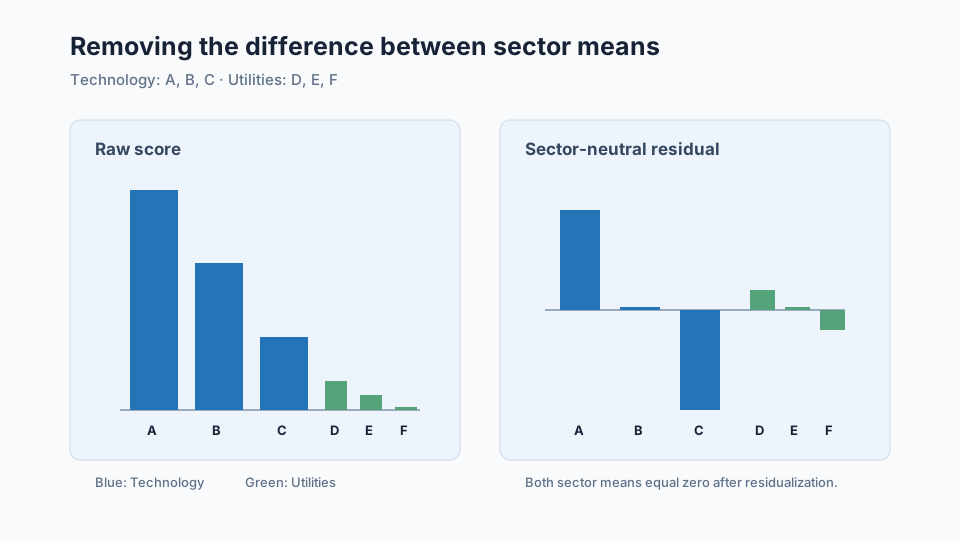
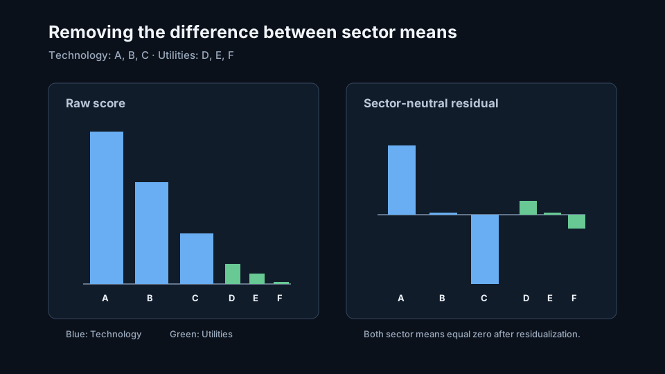
Suppose a raw signal ranks three technology stocks above three utility stocks. Within each sector, the securities also have a clear order.
Sector demeaning of a raw signal
| Security | Sector | Raw score | Sector mean | Neutralized score |
|---|---|---|---|---|
| A | Technology | 3.0 | 2.0 | +1.0 |
| B | Technology | 2.0 | 2.0 | 0.0 |
| C | Technology | 1.0 | 2.0 | −1.0 |
| D | Utilities | 0.4 | 0.2 | +0.2 |
| E | Utilities | 0.2 | 0.2 | 0.0 |
| F | Utilities | 0.0 | 0.2 | −0.2 |
For A,
\[x_A^{\perp}=3.0-\frac{3.0+2.0+1.0}{3}=1.0.\]
For D,
\[x_D^{\perp}=0.4-\frac{0.4+0.2+0.0}{3}=0.2.\]
The raw score puts every technology company above every utility. The residual score compares each company with its own sector mean. A and D are now positive, B and E neutral, and C and F negative.
Python calculation
import pandas as pd

observations = pd.DataFrame(
    {
        "sector": ["Technology", "Technology", "Technology",
                   "Utilities", "Utilities", "Utilities"],
        "raw_score": [3.0, 2.0, 1.0, 0.4, 0.2, 0.0],
    },
    index=["A", "B", "C", "D", "E", "F"],
)

sector_mean = observations.groupby("sector")["raw_score"].transform("mean")
observations["neutral_score"] = observations["raw_score"] - sector_mean

print(observations)
Scaling after neutralization
Technology has greater residual dispersion than utilities in the example. If the residuals are used directly, A and C receive five times the magnitude of D and F. A separate within-sector scaling step can equalize their dispersions:
\[z^{\perp}_{i,t} = \frac{x^{\perp}_{i,t}}{\sigma_{G(i,t),t}}.\]
Under population standard deviations, both sector triplets then become \(+1.225,0,-1.225\). This makes the sector contributions comparable, but it also amplifies a low-dispersion group. Demeaning and scaling are distinct choices.
Portfolio-level neutrality
Instead of altering the signal, a portfolio optimizer can constrain its holdings. If \(B_t\) contains sector, market-beta, and size exposures, portfolio neutrality requires
\[B_t^\top\mathbf{w}_t=\mathbf{0}.\]
For the six demeaned scores, simple unit-gross weights
\[w_i=\frac{x_i^{\perp}}{\sum_j|x_j^{\perp}|}\]
are approximately \(+41.7\%,0,-41.7\%,+8.3\%,0,-8.3\%\). Each sector's weights sum to zero. A production optimizer also accounts for covariance, liquidity, position bounds, turnover, and borrow availability.
Signal residualization asks whether the security-level relationship remains after specified exposures are removed. Portfolio constraints ask whether holdings remain neutral after risk and implementation choices. It is often useful to report both raw and neutral signal IC, then verify the realized portfolio exposures separately.
Positive, zero, and negative residuals
A positive residual lies above the value predicted by the included exposures. A negative residual lies below it. Zero means the exposure model explains the score at that date, or that the security sits exactly at its group mean in the simple categorical case.
The sign is conditional on \(B_t\). Adding size, country, or another factor can change the residual and its order. The neutralization specification therefore belongs to the factor version.
What should be neutralized?
Neutralization should follow the research question. A stock-selection signal intended to find companies within industries may remove country, sector, industry, size, and market beta. A macro factor intended to express sector rotation would lose its subject if sector exposure were removed.
Useful comparisons include raw, sector-neutral, and fully risk-neutral results. Their differences reveal where the information resides. A sign reversal after neutralization can show that the broad group relationship and the within-group relationship point in opposite directions.
Common implementation mistakes
Neutralizing with current classifications
Historical sector, industry, country, and style exposures must be those known at the observation time. Backfilled classifications can alter past residuals.
Using groups with too few observations
Small groups produce unstable means and scales. Record minimum size, combine groups under a declared hierarchy, or omit the group calculation when support is inadequate.
Removing the intended source of return
Mechanical neutralization can erase the economic relationship being studied. The exposure matrix should be justified by the hypothesis rather than copied from every other factor.
Sequentially neutralizing correlated exposures
Removing sector and then size can differ from removing size and then sector. A joint regression defines the projection once and avoids order-dependent sequential residuals.
Ignoring regression weights
Equal-weighted, capitalization-weighted, and inverse-variance regressions produce different residuals. The weights determine the orthogonality statement and should match the intended universe or risk model.
Assuming a neutral score guarantees a neutral portfolio
Covariance, bounds, missing securities, turnover limits, and execution can reintroduce exposure. Measure the final holdings against the same point-in-time exposure matrix.
Signal and portfolio evaluation
Evaluate raw and neutralized scores on the same security-date intersection. Compare rank and Pearson IC, coverage, quantile spreads, turnover, and results by group. The comparison shows whether apparent performance came from common exposure or security selection within groups.
A factor-mimicking portfolio then targets the residual score under explicit risk constraints. Walk-forward evaluation should retain the exposure matrix, regression weights, residualization coefficients, and post-trade exposure checks for each rebalance.
Frequently asked questions
Is sector ranking the same as sector neutralization?
Both can remove broad sector ordering. Ranking discards within-sector raw distance, while regression residualization retains distance after subtracting the fitted sector component. Their results can differ substantially.
Should residuals be z-scored afterward?
Often they are, particularly before combining several signals. The scale can be global or within group, and the choice changes each group's influence.
Can neutralization remove nonlinear exposure?
A linear projection removes the columns supplied to the model. Nonlinear terms, interactions, and changing relationships require additional features or another method.
Does zero sector exposure eliminate crowding risk?
No. Investors can hold similar long/short positions within every sector. Crowding, liquidity, and common exits require separate measurements and constraints.
Next reading
- Should Information Coefficient Be Sector Neutral?
- Factor exposure: security and portfolio sensitivity
- Stage 1 — From signals to a pure FMP
Sources
- Ragnar Frisch and Frederick V. Waugh, “Partial Time Regressions as Compared with Individual Trends”, Econometrica, 1933.
- M. C. Lovell, “Seasonal Adjustment of Economic Time Series and Multiple Regression Analysis”, Journal of the American Statistical Association, 1963.
- Eugene F. Fama and Kenneth R. French, “Common Risk Factors in the Returns on Stocks and Bonds”, Journal of Financial Economics, 1993.
This walkthrough is for research and educational purposes. It illustrates how strategynet.ai organizes signal evidence into factors and scenarios. It provides no recommendation, investment advice, or instruction to trade any security.
Back to Insights